5.3 The Normal Approximation to the Binomial
The binomial formula is cumbersome when the sample size (n) is large, particularly when we consider a range of observations. Consider the following example.
Example
Approximately 15% of the US population smokes cigarettes. A local government believed their community had a lower smoker rate and commissioned a survey of 400 randomly selected individuals. The survey found that only 42 of the 400 participants smoke cigarettes. If the true proportion of smokers in the community was really 15%, what is the probability of observing 42 or fewer smokers in a sample of 400 people?
The computations in the previous example are tedious, long, and near impossible if you do not have access to technology. In some cases we may use the normal distribution as an easier and faster way to estimate binomial probabilities. In general, we should avoid such work if an alternative method exists that is faster, easier, and still accurate. Recall that calculating probabilities of a range of values is much easier in the normal model. We might wonder, is it reasonable to use the normal model in place of the binomial distribution? Surprisingly, yes, if certain conditions are met.
Binomial Approximation Conditions
Consider the binomial model when the probability of a success is p = 0.10. The following figures show four hollow histograms for simulated samples from the binomial distribution using four different sample sizes: n = 10, 30, 100, 300. What happens to the shape of the distributions as the sample size increases? What distribution does the last histogram resemble?
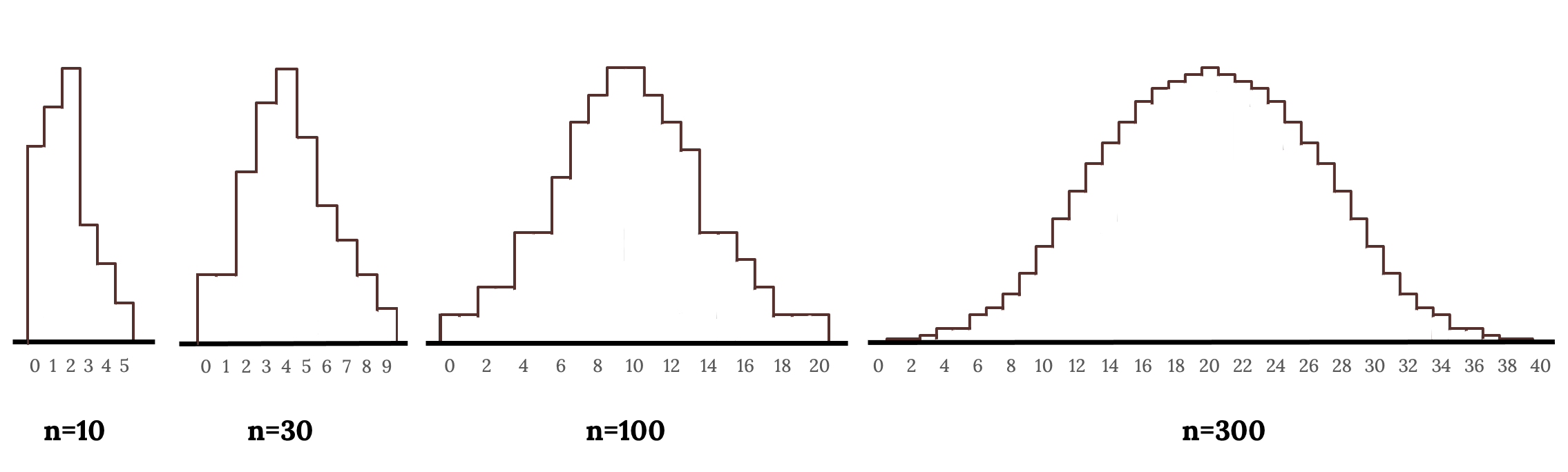
It appears the distribution is transformed from a blocky and skewed distribution into one that rather resembles the normal distribution in last hollow histogram.
The binomial distribution with probability of success p is nearly normal when the sample size n is sufficiently large that np and n(1 − p) are both at least 10. The approximate normal distribution has parameters corresponding to the mean and standard deviation of the binomial distribution:
µ = np and σ = np(1 − p)
The normal approximation may be used when computing the range of many possible successes. For instance, we may apply the normal distribution to the setting of the previous example:
Example (Continued)
Use the normal approximation to estimate the probability of observing 42 or fewer smokers in a sample of 400, if the true proportion of smokers is p = 0.15.
Already knowing that the binomial model, we then verify that both np and n(1 − p) are at least 10:
- np = 400 × 0.15 = 60 n(1 − p) = 400 × 0.85 = 340
With these conditions met, we may use the normal approximation in place of the binomial distribution using the mean and standard deviation from the binomial model:
- µ = np = 60 and σ =np(1 − p) = 7.14
We want to find the probability of observing 42 or fewer smokers using this model. Use the normal model N(µ = 60, σ = 7.14) and standardize to estimate the probability of observing 42 or fewer smokers. Your answer should be approximately equal to the solution we found in the previous of example, 0.0054.
Compute the Z-score first:
The Continuity Correction
The normal approximation to the binomial distribution tends to perform poorly when estimating the probability of a small range of counts, even when the conditions are met.
Suppose we wanted to compute the probability of observing 49, 50, or 51 smokers in 400 when p = 0.15. With such a large sample, we might be tempted to apply the normal approximation and use the range 49 to 51. However, we would find that the binomial solution and the normal approximation notably differ:
- Binomial: 0.0649
- Normal: 0.0421
We can identify the cause of this discrepancy in the next figure which shows the areas representing the binomial probability (outlined) and normal approximation (shaded). Notice that the width of the area under the normal distribution is 0.5 units too slim on both sides of the interval.
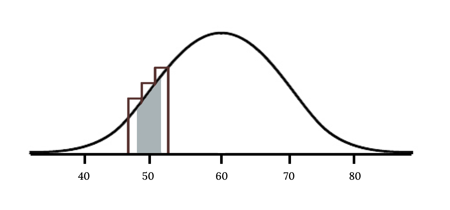
The normal approximation to the binomial distribution for intervals of values can usually be improved if cutoff values are modified slightly. The cutoff values for the lower end of a shaded region should be reduced by 0.5, and the cutoff value for the upper end should be increased by 0.5. This is called the continuity correction.
The tip to add extra area when applying the normal approximation is most often useful when examining a range of observations. In the example above, the revised normal distribution estimate is 0.0633, much closer to the exact value of 0.0649. While it is possible to also apply this correction when computing a tail area, the benefit of the modification usually disappears since the total interval is typically quite wide.
Image References
Figure 5.14: Kindred Grey (2020). “Figure 5.14.” CC BY-SA 4.0. Retrieved from https://commons.wikimedia.org/wiki/File:Figure_5.14.png
Figure 5.15: Kindred Grey via Virginia Tech (2020). “Figure 5.15” CC BY-SA 4.0. Retrieved from https://commons.wikimedia.org/wiki/File:Figure_5.15.png . Adaptation of Figure 5.39 from OpenStax Introductory Statistics (2013) (CC BY 4.0). Retrieved from https://openstax.org/books/statistics/pages/5-practice
A random variable that counts the number of successes in a fixed number (n) of independent Bernoulli trials each with probability of a success (p)
When statisticians add or subtract .5 to values to improve approximation
