6.4 The Behavior of Confidence Intervals
Once we know the basics of how to calculate a confidence interval, we also need to know how they behave. In other words how does tweaking certain parts of the equation effect the interval? Keep in mind one of the criteria that makes something a “good” statistical estimate is precision. A smaller, or more narrow interval gives us a more precise and therefore useful estimate.
Changing the Confidence Level or Sample Size
Example
Recall the previous example:
Suppose scores on exams in statistics are normally distributed with an unknown population mean and a population standard deviation of three points. A random sample of 36 scores is taken and gives a sample mean (sample mean score) of 68. Find a confidence interval estimate for the population mean exam score (the mean score on all exams).
Find a 90% confidence interval for the true (population) mean of statistics exam scores.
The 90% confidence interval is (67.1775, 68.8225).
Suppose we change the original problem by using a 95% confidence level. Find a 95% confidence interval for the true (population) mean statistics exam score.
To find the confidence interval, you need the sample mean,  , and the MoE.
- = 68
- MoE =

- σ = 3; n = 36; The confidence level is 95% (CL = 0.95).
CL = 0.95 so α = 1 – CL = 1 – 0.95 = 0.05

The area to the right of z0.025 is 0.025 and the area to the left of z0.025 is 1 – 0.025 = 0.975.

MoE = (1.96) = 0.98
– MoE = 68 – 0.98 = 67.02
+ MoE = 68 + 0.98 = 68.98
Notice that the MoE is larger for a 95% confidence level in the original problem, creating a less precise interval.
Interpretation: We estimate with 95% confidence that the true population mean for all statistics exam scores is between 67.02 and 68.98.
Alternative Interpretation
Recall the interpretation of a CI above. Ninety-five percent of all confidence intervals constructed in this way contain the true value of the population mean statistics exam score.
Comparing the results:
The 90% confidence interval is (67.18, 68.82). The 95% confidence interval is (67.02, 68.98). The 95% confidence interval is wider. If you look at the graphs, because the area 0.95 is larger than the area 0.90, it makes sense that the 95% confidence interval is wider. To be more confident that the confidence interval actually does contain the true value of the population mean for all statistics exam scores, the confidence interval necessarily needs to be wider.
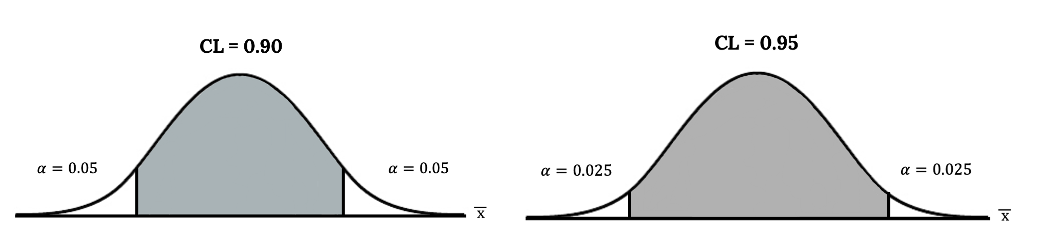
In conclusion, increasing the confidence level increases the error bound, making the confidence interval wider.
Working Backwards to Find the Error Bound or Sample Mean
When we calculate a confidence interval, we find the sample mean, calculate the error bound, and use them to calculate the confidence interval. However, sometimes when we read statistical studies, the study may state the confidence interval only. If we know the confidence interval, we can work backwards to find both the error bound and the sample mean.
- From the upper value for the interval, subtract the sample mean,
- OR, from the upper value for the interval, subtract the lower value. Then divide the difference by two.
- Subtract the error bound from the upper value of the confidence interval,
- OR, average the upper and lower endpoints of the confidence interval.
Notice that there are two methods to perform each calculation. You can choose the method that is easier to use with the information you know.
Example
Suppose we know that a confidence interval is (67.18, 68.82) and we want to find the error bound. We may know that the sample mean is 68, or perhaps our source only gave the confidence interval and did not tell us the value of the sample mean.
- If we know that the sample mean is 68: MoE = 68.82 – 68 = 0.82.
- If we don’t know the sample mean: MoE =
 = 0.82.
- If we know the error bound: = 68.82 – 0.82 = 68
- If we don’t know the error bound: =
 = 68.
= 68.
Your turn!
Suppose we know that a confidence interval is (42.12, 47.88). Find the error bound and the sample mean.
Calculating the Sample Size needed.
If researchers desire a specific margin of error, then they can use the error bound formula to calculate the required sample size.
The error bound formula for a population mean when the population standard deviation is known is
MoE = .
The formula for sample size is n =  , found by solving the error bound formula for n.
In this formula, z is  , corresponding to the desired confidence level. A researcher planning a study who wants a specified confidence level and error bound can use this formula to calculate the size of the sample needed for the study.
Example
The population standard deviation for the age of Foothill College students is 15 years. If we want to be 95% confident that the sample mean age is within two years of the true population mean age of Foothill College students, how many randomly selected Foothill College students must be surveyed?
- From the problem, we know that σ = 15 and MoE = 2.
- z = z0.025 = 1.96, because the confidence level is 95%.
- n = =
 = 216.09 using the sample size equation.
 - Use n = 217: Always round the answer UP to the next higher integer to ensure that the sample size is large enough.
Therefore, 217 Foothill College students should be surveyed in order to be 95% confident that we are within two years of the true population mean age of Foothill College students.
Example
The American Community Survey (ACS), part of the United States Census Bureau, conducts a yearly census similar to the one taken every ten years, but with a smaller percentage of participants. The most recent survey estimates with 90% confidence that the mean household income in the U.S. falls between $69,720 and $69,922.[1] Find the point estimate for mean U.S. household income and the error bound for mean U.S. household income.
The average height of young adult males has a normal distribution with standard deviation of 2.5 inches. You want to estimate the mean height of students at your college or university to within one inch with 93% confidence. How many male students must you measure?
Use the formula for MoE, solved for n:

From the statement of the problem, you know that σ = 2.5, and you need MoE = 1.
z = z0.035 = 1.812
(This is the value of z for which the area under the density curve to the right of z is 0.035.)

You need to measure at least 21 male students to achieve your goal.
Your turn!
The population standard deviation for the height of high school basketball players is three inches. If we want to be 95% confident that the sample mean height is within one inch of the true population mean height, how many randomly selected students must be surveyed?
Image References
Figure 6.10: Kindred Grey via Virginia Tech (2020). “Figure 6.8” CC BY-SA 4.0. Retrieved from https://commons.wikimedia.org/wiki/File:Figure_6.8.png . Adaptation of Figure 5.39 from OpenStax Introductory Statistics (2013) (CC BY 4.0). Retrieved from https://openstax.org/books/statistics/pages/5-practice
- American Fact Finder.” U.S. Census Bureau. Available online at http://factfinder2.census.gov/faces/nav/jsf/pages/ searchresults.xhtml?refresh=t (accessed July 2, 2013). ↵
An interval built around a point estimate for an unknown population parameter
