Chapter 5 Wrap Up
Concept Check
Section Reviews
5.1 Introduction
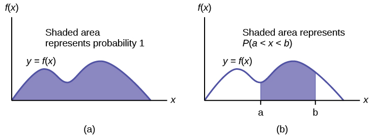
The probability density function (pdf) is used to describe probabilities for continuous random variables. The area under the density curve between two points corresponds to the probability that the variable falls between those two values. In other words, the area under the density curve between points a and b is equal to P(a < x < b). The cumulative distribution function (cdf) gives the probability as an area. If X is a continuous random variable, the probability density function (pdf), f(x), is used to draw the graph of the probability distribution. The total area under the graph of f(x) is one. The area under the graph of f(x) and between values a and b gives the probability P(a < x < b).
The cumulative distribution function (cdf) of X is defined by P (X ≤ x). It is a function of x that gives the probability that the random variable is less than or equal to x.
Probability density function (pdf) f(x):
- f(x) ≥ 0
- The total area under the curve f(x) is one.
Cumulative distribution function (cdf): P(X ≤ x)
5.2 Normal Distribution
A z-score is a standardized value. Its distribution is the standard normal, Z ~ N(0, 1). The mean of the z-scores is zero and the standard deviation is one. If z is the z-score for a value x from the normal distribution N(µ, σ) then z tells you how many standard deviations x is above (greater than) or below (less than) µ.
z = a standardized value (z-score)
mean = 0; standard deviation = 1
To find the kth percentile of X when the z-scores is known:
k = μ + (z)σ
z-score: z = 
Z = the random variable for z-scores
5.3 Normal Approximation to the Binomial
Historically, being able to compute binomial probabilities was one of the most important applications of the central limit theorem. Binomial probabilities with a small value for n(say, 20) were displayed in a table in a book. To calculate the probabilities with large values of n, you had to use the binomial formula, which could be very complicated. Using the normal approximation to the binomial distribution simplified the process. To compute the normal approximation to the binomial distribution, take a simple random sample from a population. You must meet the conditions for a binomial distribution:
- there are a certain number n of independent trials
- the outcomes of any trial are success or failure
- each trial has the same probability of a success p
Recall that if X is the binomial random variable, then X ~ B(n, p). The shape of the binomial distribution needs to be similar to the shape of the normal distribution. To ensure this, the quantities np and nq must both be greater than five (np > 5 and nq > 5; the approximation is better if they are both greater than or equal to 10). Then the binomial can be approximated by the normal distribution with mean μ = np and standard deviation σ =  . Remember that q = 1 – p. In order to get the best approximation, add 0.5 to x or subtract 0.5 from x (use x + 0.5 or x – 0.5). The number 0.5 is called the continuity correction factor and is used in the following example.
Key Terms
Try to define the terms below on your own. Scroll over any term to check your response!
5.1 Introduction
- Continuous random variable
- Probability density function (PDF)
- Cumulative distribution function (CDF)
- Uniform distribution
5.2 Normal Distribution
- Normal (Gaussian) distribution
- Probability density function (PDF)
- Empirical rule
- Standard normal distribution (SND)
- Z-score
- Quantile
5.3 Normal Approximation to the Binomial
Extra Practice
5.1 Introduction
1. What does the shaded area represent? P(___< x < ___)
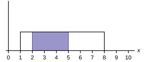
2. What does the shaded area represent? P(___< x < ___)
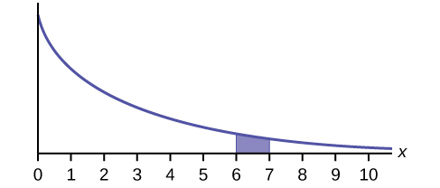
- P(6 < x < 7)
3. For a continuous probability distribution, 0 ≤ x ≤ 15. What is P(x > 15)?
4. What is the area under f(x) if the function is a continuous probability density function?
- One
5. For a continuous probability distribution, 0 ≤ x ≤ 10. What is P(x = 7)?
6. A continuous probability function is restricted to the portion between x = 0 and 7. What is P(x = 10)?
- Zero
7. f(x) for a continuous probability function is  , and the function is restricted to 0 ≤ x ≤ 5. What is P(x < 0)?
8. f(x), a continuous probability function, is equal to  , and the function is restricted to 0 ≤ x ≤ 12. What is P (0 < x < 12)?
- One
- What part of the experiment will yield discrete data?
- What part of the experiment will yield continuous data?
When age is rounded to the nearest year, do the data stay continuous, or do they become discrete? Why?
Age is a measurement, regardless of the accuracy used.
5.2 Normal Distribution
1. The mean height of 15 to 18-year-old males from Chile from 2009 to 2010 was 170 cm with a standard deviation of 6.28 cm.[1] Male heights are known to follow a normal distribution. Let X = the height of a 15 to 18-year-old male from Chile in 2009 to 2010. Then X ~ N(170, 6.28).
a. Suppose a 15 to 18-year-old male from Chile was 168 cm tall from 2009 to 2010. The z-score when x = 168 cm is z = _______. This z-score tells you that x = 168 is ________ standard deviations to the ________ (right or left) of the mean _____ (What is the mean?).
- –0.32, 0.32, left, 170
b. Suppose that the height of a 15 to 18-year-old male from Chile from 2009 to 2010 has a z-score of z = 1.27. What is the male’s height? The z-score (z = 1.27) tells you that the male’s height is ________ standard deviations to the __________ (right or left) of the mean.
- 177.98 cm, 1.27, right
2. Use the information in Number 1 to answer the following questions.
- Suppose a 15 to 18-year-old male from Chile was 176 cm tall from 2009 to 2010. The z-score when x = 176 cm is z = _______. This z-score tells you that x = 176 cm is ________ standard deviations to the ________ (right or left) of the mean _____ (What is the mean?).
- Suppose that the height of a 15 to 18-year-old male from Chile from 2009 to 2010 has a z-score of z = –2. What is the male’s height? The z-score (z = –2) tells you that the male’s height is ________ standard deviations to the __________ (right or left) of the mean.
3. In 2012, 1,664,479 students took the SAT exam. The distribution of scores in the verbal section of the SAT had a mean µ = 496 and a standard deviation σ = 114.[2] Let X = a SAT exam verbal section score in 2012. Then X ~ N(496, 114). Find the z-scores for x1 = 325 and x2 = 366.21. Interpret each z-score. What can you say about x1 = 325 and x2 = 366.21 as they compare to their respective means and standard deviations?
4. What is the z-score of x, when x = 1 and X ~ N(12,3)?
5. Some doctors believe that a person can lose five pounds, on the average, in a month by reducing his or her fat intake and by exercising consistently.[3] Suppose weight loss has a normal distribution. Let X = the amount of weight lost (in pounds) by a person in a month. Use a standard deviation of two pounds. X ~ N(5, 2). Fill in the blanks.
a. Suppose a person lost ten pounds in a month. The z-score when x = 10 pounds is z = 2.5 (verify). This z-score tells you that x = 10 is ________ standard deviations to the ________ (right or left) of the mean _____ (What is the mean?).
- This z-score tells you that x = 10 is 2.5 standard deviations to the right of the mean five.
b. Suppose a person gained three pounds (a negative weight loss). Then z = __________. This z-score tells you that x = –3 is ________ standard deviations to the __________ (right or left) of the mean.
- z = –4. This z-score tells you that x = –3 is four standard deviations to the left of the mean.
c. Suppose the random variables X and Y have the following normal distributions: X ~ N(5, 6) and Y ~ N(2, 1). If x = 17, then z = 2. (This was previously shown.) If y = 4, what is z?
- z =
 =
=  = 2 where µ = 2 and σ = 1.
 - The z-score for y = 4 is z = 2. This means that four is z = 2 standard deviations to the right of the mean. Therefore, x = 17 and y = 4 are both two (of their own) standard deviations to the right of their respective means.
6. Fill in the blanks. Jerome averages 16 points a game with a standard deviation of four points. X ~ N(16,4). Suppose Jerome scores ten points in a game. The z–score when x = 10 is –1.5. This score tells you that x = 10 is _____ standard deviations to the ______(right or left) of the mean______(What is the mean?).
7. From 1984 to 1985, the mean height of 15 to 18-year-old males from Chile was 172.36 cm, and the standard deviation was 6.34 cm.[4] Let Y = the height of 15 to 18-year-old males from 1984 to 1985. Then Y ~ N(172.36, 6.34).
The mean height of 15 to 18-year-old males from Chile from 2009 to 2010 was 170 cm with a standard deviation of 6.28 cm. Male heights are known to follow a normal distribution. Let X = the height of a 15 to 18-year-old male from Chile in 2009 to 2010. Then X ~ N(170, 6.28).
a. Find the z-scores for x = 160.58 cm and y = 162.85 cm. Interpret each z-score. What can you say about x = 160.58 cm and y = 162.85 cm as they compare to their respective means and standard deviations?
- The z-score for x = -160.58 is z = –1.5.
- The z-score for y = 162.85 is z = –1.5.
- Both x = 160.58 and y = 162.85 deviate the same number of standard deviations from their respective means and in the same direction.
8. In 2012, 1,664,479 students took the SAT exam.[5] The distribution of scores in the verbal section of the SAT had a mean µ = 496 and a standard deviation σ = 114. Let X = a SAT exam verbal section score in 2012. Then X ~ N(496, 114). Find the z-scores for x1 = 325 and x2 = 366.21. Interpret each z-score. What can you say about x1 = 325 and x2 = 366.21 as they compare to their respective means and standard deviations?
9. Suppose X has a normal distribution with mean 25 and standard deviation five. Between what values of x do 68% of the values lie?
10. The scores on a college entrance exam have an approximate normal distribution with mean, µ = 52 points and a standard deviation, σ = 11 points.
- About 68% of the y values lie between what two values? These values are ________________. The z-scores are ________________, respectively.
- About 95% of the y values lie between what two values? These values are ________________. The z-scores are ________________, respectively.
- About 99.7% of the y values lie between what two values? These values are ________________. The z-scores are ________________, respectively.
11. A bottle of water contains 12.05 fluid ounces with a standard deviation of 0.01 ounces. Define the random variable X in words. X = ____________.
- ounces of water in a bottle
12. A normal distribution has a mean of 61 and a standard deviation of 15. What is the median?
- 61
13. X ~ N(1, 2). σ = _______
- 2
14. A company manufactures rubber balls. The mean diameter of a ball is 12 cm with a standard deviation of 0.2 cm. Define the random variable X in words. X = ______________.
- diameter of a rubber ball
15. X ~ N(–4, 1). What is the median?
- –4
16. X ~ N(3, 5). σ = _______
- 5
17. X ~ N(–2, 1). μ = _______
- –2
18. What does a z-score measure?
- The number of standard deviations a value is from the mean.
19. What does standardizing a normal distribution do to the mean?
- The mean becomes zero.
20. Is X ~ N(0, 1) a standardized normal distribution? Why or why not?
- Yes because the mean is zero, and the standard deviation is one.
21. What is the z-score of x = 12, if it is two standard deviations to the right of the mean?
- z = 2
22. What is the z-score of x = 9, if it is 1.5 standard deviations to the left of the mean?
- z = –1.5
23. What is the z-score of x = –2, if it is 2.78 standard deviations to the right of the mean?
- z = 2.78
24. What is the z-score of x = 7, if it is 0.133 standard deviations to the left of the mean?
- z = –0.133
25. Suppose X ~ N(2, 6). What value of x has a z-score of three?
- x = 20
26. Suppose X ~ N(8, 1). What value of x has a z-score of –2.25?
- x = 5.75
27. Suppose X ~ N(9, 5). What value of x has a z-score of –0.5?
- x = 6.5
28. Suppose X ~ N(2, 3). What value of x has a z-score of –0.67?
- x = –0.01
29. Suppose X ~ N(4, 2). What value of x is 1.5 standard deviations to the left of the mean?
- x = 1
30. Suppose X ~ N(4, 2). What value of x is two standard deviations to the right of the mean?
- x = 8
31. Suppose X ~ N(8, 9). What value of x is 0.67 standard deviations to the left of the mean?
- x = 1.97
32. Suppose X ~ N(–1, 2). What is the z-score of x = 2?
- z = 1.5
33. Suppose X ~ N(12, 6). What is the z-score of x = 2?
- z = –1.67
34. Suppose X ~ N(9, 3). What is the z-score of x = 9?
- z = 0
35. Suppose a normal distribution has a mean of six and a standard deviation of 1.5. What is the z-score of x = 5.5?
- z ≈ –0.33
36. In a normal distribution, x = 5 and z = –1.25. This tells you that x = 5 is ____ standard deviations to the ____ (right or left) of the mean.
- 1.25, left
37. In a normal distribution, x = 3 and z = 0.67. This tells you that x = 3 is ____ standard deviations to the ____ (right or left) of the mean.
- 0.67, right
38. In a normal distribution, x = –2 and z = 6. This tells you that x = –2 is ____ standard deviations to the ____ (right or left) of the mean.
- six, right
39. In a normal distribution, x = –5 and z = –3.14. This tells you that x = –5 is ____ standard deviations to the ____ (right or left) of the mean.
- 3.14, left
40. In a normal distribution, x = 6 and z = –1.7. This tells you that x = 6 is ____ standard deviations to the ____ (right or left) of the mean.
- 1.7, left
41. About what percent of x values from a normal distribution lie within one standard deviation (left and right) of the mean of that distribution?
- about 68%
42. About what percent of the x values from a normal distribution lie within two standard deviations (left and right) of the mean of that distribution?
- about 95.45%
43. About what percent of x values lie between the second and third standard deviations (both sides)?
- about 4%
44. Suppose X ~ N(15, 3). Between what x values does 68.27% of the data lie? The range of x values is centered at the mean of the distribution (i.e., 15).
- between 12 and 18
45. Suppose X ~ N(–3, 1). Between what x values does 95.45% of the data lie? The range of x values is centered at the mean of the distribution(i.e., –3).
- between –5 and –1
46. Suppose X ~ N(–3, 1). Between what x values does 34.14% of the data lie?
- between –4 and –3 or between –3 and –2
47. About what percent of x values lie between the mean and three standard deviations?
- about 50%
48. About what percent of x values lie between the mean and one standard deviation?
- about 34.14%
49. About what percent of x values lie between the first and second standard deviations from the mean (both sides)?
- about 27%
50. About what percent of x values lie between the first and third standard deviations(both sides)?
- about 34.46%
51. The life of Sunshine CD players is normally distributed with mean of 4.1 years and a standard deviation of 1.3 years. A CD player is guaranteed for three years. We are interested in the length of time a CD player lasts.
a. Define the random variable X in words. X = _______________.
- The lifetime of a Sunshine CD player measured in years.
b. X ~ _____(_____,_____)
- X ~ N(4.1, 1.3)
52. The patient recovery time from a particular surgical procedure is normally distributed with a mean of 5.3 days and a standard deviation of 2.1 days.
a. What is the median recovery time?
- 2.7
- 5.3
- 7.4
- 2.1
- B
b. What is the z-score for a patient who takes ten days to recover?
- 1.5
- 0.2
- 2.2
- 7.3
- C
53. The length of time to find it takes to find a parking space at 9 A.M. follows a normal distribution with a mean of five minutes and a standard deviation of two minutes. If the mean is significantly greater than the standard deviation, which of the following statements is true?
- The data cannot follow the uniform distribution.
- The data cannot follow the exponential distribution..
- The data cannot follow the normal distribution.
- I only
- II only
- III only
- I, II, and III
- B
54. The heights of the 430 National Basketball Association players were listed on team rosters at the start of the 2005–2006 season. The heights of basketball players have an approximate normal distribution with mean, µ = 79 inches and a standard deviation, σ = 3.89 inches.[6] For each of the following heights, calculate the z-score and interpret it using complete sentences.
- 77 inches
- 85 inches
- If an NBA player reported his height had a z-score of 3.5, would you believe him? Explain your answer.
- Use the z-score formula. z = –0.5141. The height of 77 inches is 0.5141 standard deviations below the mean. An NBA player whose height is 77 inches is shorter than average.
- Use the z-score formula. z = 1.5424. The height 85 inches is 1.5424 standard deviations above the mean. An NBA player whose height is 85 inches is taller than average.
- Height = 79 + 3.5(3.89) = 92.615 inches, which is taller than 7 feet, 8 inches. There are very few NBA players this tall so the answer is no, not likely.
55. The systolic blood pressure (given in millimeters) of males has an approximately normal distribution with mean µ = 125 and standard deviation σ = 14. Systolic blood pressure for males follows a normal distribution.[7]
- Calculate the z-scores for the male systolic blood pressures 100 and 150 millimeters.
- If a male friend of yours said he thought his systolic blood pressure was 2.5 standard deviations below the mean, but that he believed his blood pressure was between 100 and 150 millimeters, what would you say to him?
- Use the z-score formula. 100 – 125 14 ≈ –1.8 and 100 – 125 14 ≈ 1.8 I would tell him that 2.5 standard deviations below the mean would give him a blood pressure reading of 90, which is below the range of 100 to 150.
56. Kyle’s doctor told him that the z-score for his systolic blood pressure is 1.75. Which of the following is the best interpretation of this standardized score? The systolic blood pressure (given in millimeters) of males has an approximately normal distribution with mean µ = 125 and standard deviation σ = 14. If X = a systolic blood pressure score then X ~ N (125, 14).
- Which answer(s) is/are correct?
- Kyle’s systolic blood pressure is 175.
- Kyle’s systolic blood pressure is 1.75 times the average blood pressure of men his age.
- Kyle’s systolic blood pressure is 1.75 above the average systolic blood pressure of men his age.
- Kyles’s systolic blood pressure is 1.75 standard deviations above the average systolic blood pressure for men.
- Calculate Kyle’s blood pressure.
- iv
- Kyle’s blood pressure is equal to 125 + (1.75)(14) = 149.5.
57. In 2005, 1,475,623 students heading to college took the SAT. The distribution of scores in the math section of the SAT follows a normal distribution with mean µ = 520 and standard deviation σ = 115.[8]
- Calculate the z-score for an SAT score of 720. Interpret it using a complete sentence.
- What math SAT score is 1.5 standard deviations above the mean? What can you say about this SAT score?
- For 2012, the SAT math test had a mean of 514 and standard deviation 117. The ACT math test is an alternate to the SAT and is approximately normally distributed with mean 21 and standard deviation 5.3.[9] If one person took the SAT math test and scored 700 and a second person took the ACT math test and scored 30, who did better with respect to the test they took?
Let X = an SAT math score and Y = an ACT math score.
- X = 720
 = 1.74 The exam score of 720 is 1.74 standard deviations above the mean of 520.
 - z = 1.5
The math SAT score is 520 + 1.5(115) ≈ 692.5. The exam score of 692.5 is 1.5 standard deviations above the mean of 520.  =
=  ≈ 1.59, the z-score for the SAT.
  =
=  ≈ 1.70, the z-scores for the ACT. With respect to the test they took, the person who took the ACT did better (has the higher z-score).
5.3 Normal Approximation to the Binomial
1. Suppose in a local Kindergarten through 12th grade (K – 12) school district, 53 percent of the population favor a charter school for grades K through 5. A simple random sample of 300 is surveyed.
- Find the probability that at least 150 favor a charter school.
- Find the probability that at most 160 favor a charter school.
- Find the probability that more than 155 favor a charter school.
- Find the probability that fewer than 147 favor a charter school.
- Find the probability that exactly 175 favor a charter school.
Solution:
Let X = the number that favor a charter school for grades K trough 5. X ~ B(n, p) where n = 300 and p = 0.53. Since np > 5 and nq > 5, use the normal approximation to the binomial. The formulas for the mean and standard deviation are μ = np and σ = \(\sqrt{npq}\). The mean is 159 and the standard deviation is 8.6447. The random variable for the normal distribution is Y. Y ~ N(159, 8.6447).
- For part a, you include 150 so P(X ≥ 150) has normal approximation P(Y ≥ 149.5) = 0.8641.
- For part b, you include 160 so P(X ≤ 160) has normal approximation P(Y ≤ 160.5) = 0.5689.
- For part c, you exclude 155 so P(X > 155) has normal approximation P(y > 155.5) = 0.6572.
- For part d, you exclude 147 so P(X < 147) has normal approximation P(Y < 146.5) = 0.0741.
- For part e,P(X = 175) has normal approximation P(174.5 < Y < 175.5) = 0.0083.
2. In a city, 46 percent of the population favor the incumbent, Dawn Morgan, for mayor. A simple random sample of 500 is taken. Using the continuity correction factor, find the probability that at least 250 favor Dawn Morgan for mayor.
References
Image References
Figure 5.16: Figure 5.21 from OpenStax Introductory Business Statistics (2012) (CC BY 4.0). Retrieved from https://openstax.org/books/introductory-business-statistics/pages/5-chapter-review
Figure 5.17: Figure 5.26 from OpenStax Introductory Business Statistics (2012) (CC BY 4.0). Retrieved from https://openstax.org/books/introductory-business-statistics/pages/5-practice
Figure 5.18: Figure 5.27 from OpenStax Introductory Business Statistics (2012) (CC BY 4.0). Retrieved from https://openstax.org/books/introductory-business-statistics/pages/5-practice
Text
“Blood Pressure of Males and Females.” StatCruch, 2013. Available online at http://www.statcrunch.com/5.0/viewreport.php?reportid=11960 (accessed May 14, 2013).
“The Use of Epidemiological Tools in Conflict-affected populations: Open-access educational resources for policy-makers: Calculation of z-scores.” London School of Hygiene and Tropical Medicine, 2009. Available online at http://conflict.lshtm.ac.uk/page_125.htm (accessed May 14, 2013).
“2012 College-Bound Seniors Total Group Profile Report.” CollegeBoard, 2012. Available online at http://media.collegeboard.com/digitalServices/pdf/research/TotalGroup-2012.pdf (accessed May 14, 2013).
“Digest of Education Statistics: ACT score average and standard deviations by sex and race/ethnicity and percentage of ACT test takers, by selected composite score ranges and planned fields of study: Selected years, 1995 through 2009.” National Center for Education Statistics. Available online at http://nces.ed.gov/programs/digest/d09/tables/dt09_147.asp (accessed May 14, 2013).
Data from the San Jose Mercury News.
Data from The World Almanac and Book of Facts.
“List of stadiums by capacity.” Wikipedia. Available online at https://en.wikipedia.org/wiki/List_of_stadiums_by_capacity (accessed May 14, 2013).
Data from the National Basketball Association. Available online at www.nba.com (accessed May 14, 2013).
- Data from The World Almanac and Book of Facts. ↵
- “2012 College-Bound Seniors Total Group Profile Report.” CollegeBoard, 2012. Available online at http://media.collegeboard.com/digitalServices/pdf/research/TotalGroup-2012.pdf (accessed May 14, 2013). ↵
- McDougall, John A. The McDougall Program for Maximum Weight Loss. Plume, 1995. ↵
- Data from The World Almanac and Book of Facts. ↵
- “2012 College-Bound Seniors Total Group Profile Report.” CollegeBoard, 2012. Available online at http://media.collegeboard.com/digitalServices/pdf/research/TotalGroup-2012.pdf (accessed May 14, 2013). ↵
- Data from the National Basketball Association. Available online at www.nba.com (accessed May 14, 2013). ↵
- “Blood Pressure of Males and Females.” StatCruch, 2013. Available online at http://www.statcrunch.com/5.0/ viewreport.php?reportid=11960 (accessed May 14, 2013). ↵
- “2012 College-Bound Seniors Total Group Profile Report.” CollegeBoard, 2012. Available online at http://media.collegeboard.com/digitalServices/pdf/research/TotalGroup-2012.pdf (accessed May 14, 2013). ↵
- “Digest of Education Statistics: ACT score average and standard deviations by sex and race/ethnicity and percentage of ACT test takers, by selected composite score ranges and planned fields of study: Selected years, 1995 through 2009.” National Center for Education Statistics. Available online at http://nces.ed.gov/programs/digest/d09/tables/dt09_147.asp (accessed May 14, 2013). ↵
A random variable (RV) whose outcomes are measured as an uncountable, infinite, number of values
A function that defines a continuous random variable, and the likelihood of an outcome
A function that gives the probability that a random variable takes a value less than or equal to x
A probability distribution in which all outcomes are equally likely
A commonly used symmetric, unimodal, bell-shaped, continuous probability distribution
Roughly 68% of values are within 1 standard deviation of the mean, roughly 95% of values are within 2 standard deviations of the mean, and 99.7% of values are within 3 standard deviations of the mean
A normal random variable with a mean of 0 and standard deviation of 1 which z-scores follow; denoted N(0, 1)
A measure of location that tells us how many standard deviations a value is above or below the mean
Points in a distribution that relate to the rank order of values in that distribution
A random variable that counts the number of successes in a fixed number (n) of independent Bernoulli trials each with probability of a success (p)
When statisticians add or subtract .5 to values to improve approximation
