8.3 Inference for Two Sample Proportions
Comparing two proportions, like comparing two means, is also very common when we are working with categorical data. If our parameter of inference is p1-p2, then we can estimate it with  –
– 
When conducting inference on two independent population proportions, the following characteristics should be present:
- The two independent samples are simple random samples that are independent.
- The number of successes is at least five, and the number of failures is at least five, for each of the samples.
- Growing literature states that the population must be at least ten or 20 times the size of the sample. This keeps each population from being over-sampled and causing incorrect results.
Sampling Distribution of the Difference in Two Proportions
We can build a sampling distribution for – similar to how we did for the difference in two independent sample means. The difference of two proportions follows an approximate normal distribution. We will wait to show the standard error and sampling distribution because we calculate it slightly differently for hypothesis tests and confidence intervals
Hypothesis Test for the Difference in Two Proportions
If two estimated proportions are different, it may be due to a difference in the populations or it may be due to chance. A hypothesis test can help determine if a difference in the estimated proportions reflects a difference in the population proportions. A confidence Interval can then
Generally, the null hypothesis states that the two proportions are the same, that is, H0: p1 = p2. Since we are assuming there is no difference in the null, we can use both samples to estimate the pooled proportion, pp , calculated as follows:

We can use this pooled proportion in the calculation of our Z test statistic:

Example
Two types of medication for hives are being tested to determine if there is a difference in the proportions of adult patient reactions. Twenty out of a random sample of 200 adults given medication A still had hives 30 minutes after taking the medication. Twelve out of another random sample of 200 adults given medication B still had hives 30 minutes after taking the medication. Test at a 1% level of significance.
Graph:
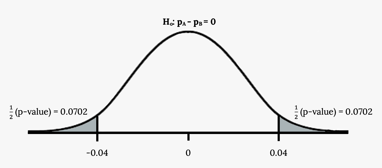
Your turn!
Two types of valves are being tested to determine if there is a difference in pressure tolerances. Fifteen out of a random sample of 100 of Valve A cracked under 4,500 psi. Six out of a random sample of 100 of Valve B cracked under 4,500 psi. Test at a 5% level of significance.
Confidence Intervals for the Difference in Two Proportions
Once we have identified we have a difference in a two sample test, we may want to estimate it. Our confidence interval would be of the form:

Where our point estimate is –
And the MoE is made up of:
 ,
, is the z critical value with area to the right equal to
- And SE

- In the SE will we estimate p1 with and p2 with if we do not know them.
Putting that all together our formula for a CI to estimate the difference in two proportions will be:
– 
Image References
Figure 8.8: Kindred Grey via Virginia Tech (2020). “Figure 8.8” CC BY-SA 4.0. Retrieved from https://commons.wikimedia.org/wiki/File:Figure_8.8.png . Adaptation of Figure 5.39 from OpenStax Introductory Statistics (2013) (CC BY 4.0). Retrieved from https://openstax.org/books/statistics/pages/5-practice
Data that describes qualities, or puts individuals into categories
Using information from a sample to answer a question, or generalize, about a population
The occurrence of one event has no effect on the probability of the occurrence of another event
The number of individuals that have a characteristic we are interested in divided by the total number in the population
The probability distribution of a statistic at a given sample size
The standard deviation of a sampling distribution
Estimate of the common value of p1 and p2
An interval built around a point estimate for an unknown population parameter
The value that is calculated from a sample used to estimate an unknown population parameter
