9.5 Inference for Regression
The previous sections in this chapter have focused on linear regression as a tool for summarizing trends in data and making predictions. These numerical summaries are analogous to the methods discussed in Chapter 2 for displaying and summarizing data. Regression is also used to make inferences about a population. The same ideas covered in Chapters 6-8 about using data from a sample to draw inferences about population parameters can also apply to regression. Previously, the goal was to draw inference about a population parameter such as µ or p. In regression, the population parameter of interest is typically the slope parameter β. Inference about the intercept term is rare, but can be done where the vertical intercept is meaningful.
- r is an unbiased point estimate of the population correlation, ρ
- a is an unbiased estimate for the Y-intercept, β0
- b is an unbiased estimate for slope, β1
- ŷ is an unbiased estimate for mean response, µy
So a set of ordered pairs (x, y) used when fitting a least squares regression line are assumed to have been sampled from a population in which the relationship between the explanatory and response variables with the following equation:
Y = β0 + β1X + ε
Where ε, the error, is assumed to have a normal distribution with mean 0 and standard deviation σ
(ε ∼ N(0, σ)).
Inference for regression Assumptions:
Like any inferential technique, we need to meet an underlying set of assumptions in order to appropriately use them.
- Like always, the data are collected from a well-designed, random sample or randomized experiment.
- The relationship is Linear
-
The standard deviation of y is the same for all values of x.
-
The response y varies Normally around its mean
- The residual errors are independent (no pattern).
You can check most of these using a residual plot.
Regression Standard Errors
Statistical software is typically used to obtain t-statistics and p-values for inference with regression, since using the formulas for calculating standard error can be cumbersome. However, the formulas are displayed below
The standard error of the residuals is:
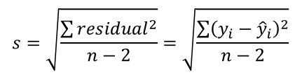
Notice n-2 degrees of freedom!
Using that to calculate the standard error of the sampling distribution of the slope, b:
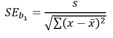
We can use this to do perform inference on the slope.
Inference on the slope
We now know the sampling distribution of the slope, b, is:
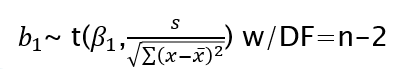
Hypothesis tests and confidence intervals for regression parameters have the same basic form as tests and intervals about population means.
Hypothesis tests on the slope
We often times want to check for the significance of the slope of a regression equation. In other words is the slope actually different from 0? In this case your Null Hypothesis would be:
H0 : β1 = 0
We can use the test statistic:

- Since our slope, b, is calculated directly from the correlation coefficient, r, testing for a significant slope is essentially the same as testing for significance of the correlation coefficient
- It is possible to test for values other than 0 in the Null
Confidence Intervals for the slope
Finally, we may also be interested in estimating the true value of the slope with a confidence interval. We know the sampling distribution of the slope and can follow the same format we are familiar with for a Confidence Interval for the slope, b:
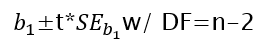
We interpret this interval similar to how we have before. For instance you could be 95% confident the interval you’ve created captures the true value of the slope.
