Chapter 8 Wrap Up

Adapted by John Morgan Russell; from Barbara Illowsky and Susan Dean, David Diez, Mine Cetinkaya-Rundel and Christopher D. Barr; Julie Vu and David Harrington

Chapter 8 Wrap Up

Concept Check

Section Reviews

8.1 Inference for 2 Dependent Samples (Matched Pairs)

A hypothesis test for matched or paired samples (t-test) has these characteristics:

Test the differences by subtracting one measurement from the other measurement
Random Variable: ${\overline{x}}_{d}$ = mean of the differences
Distribution: Student’s-t distribution with n – 1 degrees of freedom
If the number of differences is small (less than 30), the differences must follow a normal distribution.
Two samples are drawn from the same set of objects.
Samples are dependent.

Test Statistic (t-score): t = $\frac{{\overline{x}}_{d}-{\mu }_{d}}{\left(\frac{{s}_{d}}{\sqrt{n}}\right)}$ where: ${\overline{x}}_{d}$ is the mean of the sample differences. μ_d is the mean of the population differences. s_d is the sample standard deviation of the differences. n is the sample size.

8.2 Inference for 2 Independent Sample Means

A hypothesis test of two population means from independent samples where the population standard deviations are known (typically approximated with the sample standard deviations), will have these characteristics:

Random variable: ${\overline{X}}_{1}-{\overline{X}}_{2}$ = the difference of the means
Distribution: normal distribution

Normal Distribution:
${\overline{X}}_{1}-{\overline{X}}_{2}\sim N\left[{\mu }_{1}-{\mu }_{2},\sqrt{\frac{{\left({\sigma }_{1}\right)}^{2}}{{n}_{1}}+\frac{{\left({\sigma }_{2}\right)}^{2}}{{n}_{2}}}\right]$ .

Test Statistic (z-score):

$z=\frac{\left({\overline{x}}_{1}-{\overline{x}}_{2}\right)-\left({\mu }_{1}-{\mu }_{2}\right)}{\sqrt{\frac{{\left({\sigma }_{1}\right)}^{2}}{{n}_{1}}+\frac{{\left({\sigma }_{2}\right)}^{2}}{{n}_{2}}}}$

And Null hypothesis Generally H₀: µ₁ – µ₂ = 0 or µ₁ = µ₂

where:
σ₁ and σ₂ are the known population standard deviations. n₁ and n₂ are the sample sizes. ${\overline{x}}_{1}$ and ${\overline{x}}_{2}$ are the sample means. μ₁ and μ₂ are the population means.

However, most likely we do not know σ₁ and σ₂so we usually use the t distribution with Test Statistic:

$t=\frac{\left({\overline{x}}_{1}-{\overline{x}}_{2}\right)-\left({\mu }_{1}-{\mu }_{2}\right)}{\sqrt{\frac{{\left({s }_{1}\right)}^{2}}{{n}_{1}}+\frac{{\left({s}_{2}\right)}^{2}}{{n}_{2}}}}$

8.3 Inference for 2 Sample Proportions

Test of two population proportions from independent samples

Random variable: p₁-p₂ , the difference between the two estimated proportions
Distribution: normal distribution

We oftne use the “Pooled” Proportion:

p_p = $\frac{{x}_{1}+{x}_{2}}{{n}_{1}+{n}_{2}}$

Distribution for the differences:
${\hat{p}}_{1}-{\hat{p}}_{2}\sim N\left[0,\sqrt{{p}_{p}\left(1-{p}_{p}\right)\left(\frac{1}{{n}_{1}}+\frac{1}{{n}_{2}}\right)}\right]$

With Test Statistic:

$z=\frac{\left(\hat{p}_{1}-\hat{p}_{2}\right)}{\sqrt{{p}_{p}\left(1-{p}_{p}\right)\left(\frac{1}{{n}_{1}}+\frac{1}{{n}_{2}}\right)}}$

And Null hypothesis H₀: p_A = p_Bor H₀: p_A − p_B = 0.

where:

p̂₁ and p̂₂ are the sample proportions, p₁ and p₂ are the population proportions,

P_p is the pooled proportion, and n₁ and n₂ are the sample sizes.

Key Terms

Try to define the terms below on your own. Scroll over any term to check your response!

8.1 Inference for 2 Dependent Samples (Matched Pairs)

Placebo
Inference
Means
Proportions
Quantitative data
Categorical data
Independent
Matched pairs
Population mean difference
Sampling distribution
Point estimate

8.2 Inference for 2 Independent Sample Means

Independent
Quantitative data
Parameter
Difference in means
Point estimate
Standard error
Inference
Sampling distribution
Test statistic
Confidence interval
Outliers
Degrees of freedom

Extra Practice

8.1 Inference for 2 Dependent Samples (Matched Pairs)

1. Seven eighth graders at Kennedy Middle School measured how far they could push the shot-put with their dominant (writing) hand and their weaker (non-writing) hand. They thought that they could push equal distances with either hand. The data were collected and recorded below.

Figure 8.9
Distance (in feet) using	Student 1	Student 2	Student 3	Student 4	Student 5	Student 6	Student 7
Dominant Hand	30	26	34	17	19	26	20
Weaker Hand	28	14	27	18	17	26	16

Conduct a hypothesis test to determine whether the mean difference in distances between the children’s dominant versus weaker hands is significant.

Record the differences data. Calculate the differences by subtracting the distances with the weaker hand from the distances with the dominant hand. The data for the differences are: {2, 12, 7, –1, 2, 0, 4}. The differences have a normal distribution.

Using the differences data, calculate the sample mean and the sample standard deviation.

${\overline{x}}_{d}$ = 3.71, ${s}_{d}$ = 4.5.

Random variable: ${\overline{X}}_{d}$ = mean difference in the distances between the hands.

Distribution for the hypothesis test:t₆

H₀: μ_d = 0 H_a: μ_d ≠ 0

Graph:

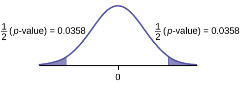
This is a normal distribution curve with mean equal to zero. Both the right and left tails of the curve are shaded. Each tail represents 1/2(p-value) = 0.0358. — Figure 8.10

Calculate the p-value: The p-value is 0.0716 (using the data directly).

(test statistic = 2.18. p-value = 0.0719 using $\left({\overline{x}}_{d}=3.71,\text{ }{s}_{d}=4.5.\right)$

Decision: Assume α = 0.05. Since α < p-value, Do not reject H₀.

Conclusion: At the 5% level of significance, from the sample data, there is not sufficient evidence to conclude that there is a difference in the children’s weaker and dominant hands to push the shot-put.

2. Five ball players think they can throw the same distance with their dominant hand (throwing) and off-hand (catching hand). The data were collected and recorded below. Conduct a hypothesis test to determine whether the mean difference in distances between the dominant and off-hand is significant. Test at the 5% level.

Figure 8.11
	Player 1	Player 2	Player 3	Player 4	Player 5
Dominant Hand	120	111	135	140	125
Off-hand	105	109	98	111	99

3. A study was conducted to test the effectiveness of a software patch in reducing system failures over a six-month period. Results for randomly selected installations are shown below. The “before” value is matched to an “after” value, and the differences are calculated. The differences have a normal distribution. Test at the 1% significance level.

Figure 8.12
Installation	A	B	C	D	E	F	G	H
Before	3	6	4	2	5	8	2	6
After	1	5	2	0	1	0	2	2

a. What is the random variable?

the mean difference of the system failures

b. State the null and alternative hypotheses.

c. What is the p-value?

0.0067

d. Draw the graph of the p-value.

e. What conclusion can you draw about the software patch?

With a p-value 0.0067, we can reject the null hypothesis. There is enough evidence to support that the software patch is effective in reducing the number of system failures.

4. A study was conducted to test the effectiveness of a juggling class. Before the class started, six subjects juggled as many balls as they could at once. After the class, the same six subjects juggled as many balls as they could. The differences in the number of balls are calculated. The differences have a normal distribution. Test at the 1% significance level.

Figure 8.13
Subject	A	B	C	D	E	F
Before	3	4	3	2	4	5
After	4	5	6	4	5	7

a. State the null and alternative hypotheses.

b. What is the p-value?

0.0021

c. What is the sample mean difference?

d. Draw the graph of the p-value.

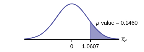
This is a normal distribution curve with mean equal to zero. The values 0 and 1.67 are labeled on the horiztonal axis. A vertical line extends from 1.67 to the curve. The region under the curve to the right of the line is shaded to represent p-value = 0.0021. — Figure 8.14

e. What conclusion can you draw about the juggling class?

5. A doctor wants to know if a blood pressure medication is effective. Six subjects have their blood pressures recorded. After twelve weeks on the medication, the same six subjects have their blood pressure recorded again. For this test, only systolic pressure is of concern. Test at the 1% significance level.

Figure 8.15
Patient	A	B	C	D	E	F
Before	161	162	165	162	166	171
After	158	159	166	160	167	169

a. State the null and alternative hypotheses.

H₀: μ_d ≥ 0
H_a: μ_d < 0

b. What is the test statistic?

c. What is the p-value?

0.0699

d. What is the sample mean difference?

e. What is the conclusion?

We decline to reject the null hypothesis. There is not sufficient evidence to support that the medication is effective.

DIRECTIONS: For each of the word problems, use a solution sheet to do the hypothesis test. The solution sheet is found in Appendix E. Please feel free to make copies of the solution sheets. For the online version of the book, it is suggested that you copy the .doc or the .pdf files.

Note: If you are using a Student’s t-distribution for the homework problems, including for paired data, you may assume that the underlying population is normally distributed. (When using these tests in a real situation, you must first prove that assumption, however.)

6. Ten individuals went on a low–fat diet for 12 weeks to lower their cholesterol. The data are recorded below. Do you think that their cholesterol levels were significantly lowered?

Figure 8.16
Starting cholesterol level	Ending cholesterol level
140	140
220	230
110	120
240	220
200	190
180	150
190	200
360	300
280	300
260	240

p-value = 0.1494
At the 5% significance level, there is insufficient evidence to conclude that the medication lowered cholesterol levels after 12 weeks.

7. A new AIDS prevention drug was tried on a group of 224 HIV positive patients. Forty-five patients developed AIDS after four years. In a control group of 224 HIV positive patients, 68 developed AIDS after four years. We want to test whether the method of treatment reduces the proportion of patients that develop AIDS after four years or if the proportions of the treated group and the untreated group stay the same.

Let the subscript t = treated patient and ut = untreated patient.

The appropriate hypotheses are:

H₀: p_t < p_ut and H_a: p_t ≥ p_ut
H₀: p_t ≤ p_ut and H_a: p_t > p_ut
H₀: p_t = p_ut and H_a: p_t ≠ p_ut
H₀: p_t = p_ut and H_a: p_t < p_ut

If the p-value is 0.0062 what is the conclusion (use α = 0.05)?

The method has no effect.
There is sufficient evidence to conclude that the method reduces the proportion of HIV positive patients who develop AIDS after four years.
There is sufficient evidence to conclude that the method increases the proportion of HIV positive patients who develop AIDS after four years.
There is insufficient evidence to conclude that the method reduces the proportion of HIV positive patients who develop AIDS after four years.

Solution: b

8. An experiment is conducted to show that blood pressure can be consciously reduced in people trained in a “biofeedback exercise program.” Six subjects were randomly selected and blood pressure measurements were recorded before and after the training. The difference between blood pressures was calculated (after – before) producing the following results: ${\overline{x}}_{d}$ = −10.2 s_d = 8.4. Using the data, test the hypothesis that the blood pressure has decreased after the training.

The distribution for the test is:

t₅
t₆
N(−10.2, 8.4)
N(−10.2, $\frac{8.4}{\sqrt{6}}$

If α = 0.05, the p-value and the conclusion are

0.0014; There is sufficient evidence to conclude that the blood pressure decreased after the training.
0.0014; There is sufficient evidence to conclude that the blood pressure increased after the training.
0.0155; There is sufficient evidence to conclude that the blood pressure decreased after the training.
0.0155; There is sufficient evidence to conclude that the blood pressure increased after the training.

Solution: c

9. A golf instructor is interested in determining if her new technique for improving players’ golf scores is effective. She takes four new students. She records their 18-hole scores before learning the technique and then after having taken her class. She conducts a hypothesis test. The data are as follows.

Figure 8.17
	Player 1	Player 2	Player 3	Player 4
Mean score before class	83	78	93	87
Mean score after class	80	80	86	86

The correct decision is:

Reject H₀.
Do not reject the H₀.

10. A local cancer support group believes that the estimate for new female breast cancer cases in the south is higher in 2013 than in 2012. The group compared the estimates of new female breast cancer cases by southern state in 2012 and in 2013. The results are shown below.

Figure 8.18
Southern States	2012	2013
Alabama	3,450	3,720
Arkansas	2,150	2,280
Florida	15,540	15,710
Georgia	6,970	7,310
Kentucky	3,160	3,300
Louisiana	3,320	3,630
Mississippi	1,990	2,080
North Carolina	7,090	7,430
Oklahoma	2,630	2,690
South Carolina	3,570	3,580
Tennessee	4,680	5,070
Texas	15,050	14,980
Virginia	6,190	6,280

Test: two matched pairs or paired samples (t-test)

Random variable: ${\overline{X}}_{d}$

Distribution: t₁₂

H₀: μ_d = 0 H_a: μ_d > 0

The mean of the differences of new female breast cancer cases in the south between 2013 and 2012 is greater than zero. The estimate for new female breast cancer cases in the south is higher in 2013 than in 2012.

Graph: right-tailed

p-value: 0.0004

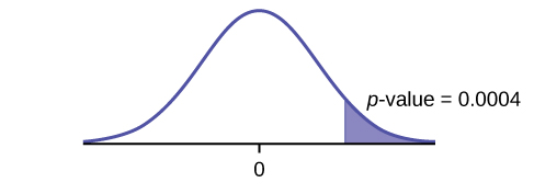
This is a normal distribution curve with mean equal to zero. A vertical line near the tail of the curve to the right of zero extends from the axis to the curve. The region under the curve to the right of the line is shaded representing p-value = 0.0004. — Figure 8.19

Decision: Reject H₀

Conclusion: At the 5% level of significance, from the sample data, there is sufficient evidence to conclude that there was a higher estimate of new female breast cancer cases in 2013 than in 2012.

11. A traveler wanted to know if the prices of hotels are different in the ten cities that he visits the most often. The list of the cities with the corresponding hotel prices for his two favorite hotel chains is shown below. Test at the 1% level of significance.

Figure 8.20
Cities	Hyatt Regency prices in dollars	Hilton prices in dollars
Atlanta	107	169
Boston	358	289
Chicago	209	299
Dallas	209	198
Denver	167	169
Indianapolis	179	214
Los Angeles	179	169
New York City	625	459
Philadelphia	179	159
Washington, DC	245	239

12. A politician asked his staff to determine whether the underemployment rate in the northeast decreased from 2011 to 2012. The results are shown below.

Figure 8.21
Northeastern States	2011	2012
Connecticut	17.3	16.4
Delaware	17.4	13.7
Maine	19.3	16.1
Maryland	16.0	15.5
Massachusetts	17.6	18.2
New Hampshire	15.4	13.5
New Jersey	19.2	18.7
New York	18.5	18.7
Ohio	18.2	18.8
Pennsylvania	16.5	16.9
Rhode Island	20.7	22.4
Vermont	14.7	12.3
West Virginia	15.5	17.3

Test: matched or paired samples (t-test)

Difference data: {–0.9, –3.7, –3.2, –0.5, 0.6, –1.9, –0.5, 0.2, 0.6, 0.4, 1.7, –2.4, 1.8}

Random Variable: ${\overline{X}}_{d}$

Distribution: H₀: μ_d = 0 H_a: μ_d < 0

The mean of the differences of the rate of underemployment in the northeastern states between 2012 and 2011 is less than zero. The underemployment rate went down from 2011 to 2012.

Graph: left-tailed.

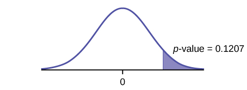
p-value: 0.1207

Decision: Do not reject H₀.

Conclusion: At the 5% level of significance, from the sample data, there is not sufficient evidence to conclude that there was a decrease in the underemployment rates of the northeastern states from 2011 to 2012.

13-22. Indicate which of the following choices best identifies the hypothesis test.

independent group means, population standard deviations and/or variances known
independent group means, population standard deviations and/or variances unknown
matched or paired samples
single mean
two proportions
single proportion

13. A powder diet is tested on 49 people, and a liquid diet is tested on 36 different people. The population standard deviations are two pounds and three pounds, respectively. Of interest is whether the liquid diet yields a higher mean weight loss than the powder diet.

14. Use the list from 13 to choose the best hypothesis test. A new chocolate bar is taste-tested on consumers. Of interest is whether the proportion of children who like the new chocolate bar is greater than the proportion of adults who like it.

e

15. Use the list from 13 to choose the best hypothesis test. The mean number of English courses taken in a two–year time period by male and female college students is believed to be about the same. An experiment is conducted and data are collected from nine males and 16 females.

16. Use the list from 13 to choose the best hypothesis test. A football league reported that the mean number of touchdowns per game was five. A study is done to determine if the mean number of touchdowns has decreased.

d

17. Use the list from 13 to choose the best hypothesis test. A study is done to determine if students in the California state university system take longer to graduate than students enrolled in private universities. One hundred students from both the California state university system and private universities are surveyed. From years of research, it is known that the population standard deviations are 1.5811 years and one year, respectively.

18. Use the list from 13 to choose the best hypothesis test. According to a YWCA Rape Crisis Center newsletter, 75% of rape victims know their attackers. A study is done to verify this.

f

19. Use the list from 13 to choose the best hypothesis test. According to a recent study, U.S. companies have a mean maternity-leave of six weeks.

20. Use the list from 13 to choose the best hypothesis test. A recent drug survey showed an increase in use of drugs and alcohol among local high school students as compared to the national percent. Suppose that a survey of 100 local youths and 100 national youths is conducted to see if the proportion of drug and alcohol use is higher locally than nationally.

e

21. Use the list from 13 to choose the best hypothesis test. A new SAT study course is tested on 12 individuals. Pre-course and post-course scores are recorded. Of interest is the mean increase in SAT scores. The following data are collected:

Figure 8.23
Pre-course score	Post-course score
1	300
960	920
1010	1100
840	880
1100	1070
1250	1320
860	860
1330	1370
790	770
990	1040
1110	1200
740	850

22. Use the list from 13 to choose the best hypothesis test. University of Michigan researchers reported in the Journal of the National Cancer Institute that quitting smoking is especially beneficial for those under age 49. In this American Cancer Society study, the risk (probability) of dying of lung cancer was about the same as for those who had never smoked.^[1]

f

23. Lesley E. Tan investigated the relationship between left-handedness vs. right-handedness and motor competence in preschool children. Random samples of 41 left-handed preschool children and 41 right-handed preschool children were given several tests of motor skills to determine if there is evidence of a difference between the children based on this experiment. The experiment produced the means and standard deviations shown below. Determine the appropriate test and best distribution to use for that test.

Figure 8.24
	Left-handed	Right-handed
Sample size	41	41
Sample mean	97.5	98.1
Sample standard deviation	17.5	19.2

Two independent means, normal distribution
Two independent means, Student’s-t distribution
Matched or paired samples, Student’s-t distribution
Two population proportions, normal distribution

24. A golf instructor is interested in determining if her new technique for improving players’ golf scores is effective. She takes four (4) new students. She records their 18-hole scores before learning the technique and then after having taken her class. She conducts a hypothesis test. The data are:

Figure 8.25
	Player 1	Player 2	Player 3	Player 4
Mean score before class	83	78	93	87
Mean score after class	80	80	86	86

This is:

a test of two independent means.
a test of two proportions.
a test of a single mean.
a test of a single proportion.

Solution: a

8.2 Inference for 2 Independent Sample Means

Independent groups, population standard deviations known: The mean lasting time of two competing floor waxes is to be compared. Twenty floors are randomly assigned to test each wax. Both populations have a normal distributions. The data are recorded in (Figure).

Wax	Sample Mean Number of Months Floor Wax Lasts	Population Standard Deviation
1	3	0.33
2	2.9	0.36

Does the data indicate that wax 1 is more effective than wax 2? Test at a 5% level of significance.

This is a test of two independent groups, two population means, population standard deviations known.

Random Variable: ${\overline{X}}_{1}\text{- }{\overline{X}}_{2}$ = difference in the mean number of months the competing floor waxes last.

H₀: μ₁ ≤ μ₂

H_a: μ₁ > μ₂

The words “is more effective” says that wax 1 lasts longer than wax 2, on average. “Longer” is a “>” symbol and goes into H_a. Therefore, this is a right-tailed test.

Distribution for the test: The population standard deviations are known so the distribution is normal. Using the formula, the distribution is:

${\overline{X}}_{1}-{\overline{X}}_{2}~N\left(0,\sqrt{\frac{{0.33}^{2}}{20}+\frac{{0.36}^{2}}{20}}\right)$

Since μ₁ ≤ μ₂ then μ₁ – μ₂ ≤ 0 and the mean for the normal distribution is zero.

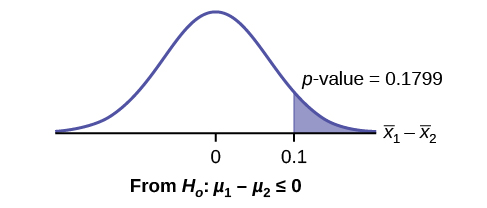
Calculate the p-value using the normal distribution:p-value = 0.1799

Graph:

This is a normal distribution curve with mean equal to zero. The values 0 and 0.1 are labeled on the horiztonal axis. A vertical line extends from 0.1 to the curve. The region under the curve to the right of the line is shaded to represent p-value = 0.1799.

${\overline{X}}_{1}$ – ${\overline{X}}_{2}$ = 3 – 2.9 = 0.1

Compare α and the p-value:α = 0.05 and p-value = 0.1799. Therefore, α < p-value.

Make a decision: Since α < p-value, do not reject H₀.

Conclusion: At the 5% level of significance, from the sample data, there is not sufficient evidence to conclude that the mean time wax 1 lasts is longer (wax 1 is more effective) than the mean time wax 2 lasts.

Try It

The means of the number of revolutions per minute of two competing engines are to be compared. Thirty engines are randomly assigned to be tested. Both populations have normal distributions. (Figure) shows the result. Do the data indicate that Engine 2 has higher RPM than Engine 1? Test at a 5% level of significance.

Engine	Sample Mean Number of RPM	Population Standard Deviation
1	1,500	50
2	1,600	60

Use the following information to answer the next five exercises. The mean speeds of fastball pitches from two different baseball pitchers are to be compared. A sample of 14 fastball pitches is measured from each pitcher. The populations have normal distributions. (Figure) shows the result. Scouters believe that Rodriguez pitches a speedier fastball.

Pitcher	Sample Mean Speed of Pitches (mph)	Population Standard Deviation
Wesley	86	3
Rodriguez	91	7

What is the random variable?

The difference in mean speeds of the fastball pitches of the two pitchers

State the null and alternative hypotheses.

What is the test statistic?

–2.46

What is the p-value?

At the 1% significance level, what is your conclusion?

At the 1% significance level, we can reject the null hypothesis. There is sufficient data to conclude that the mean speed of Rodriguez’s fastball is faster than Wesley’s.

Use the following information to answer the next five exercises. A researcher is testing the effects of plant food on plant growth. Nine plants have been given the plant food. Another nine plants have not been given the plant food. The heights of the plants are recorded after eight weeks. The populations have normal distributions. The following table is the result. The researcher thinks the food makes the plants grow taller.

Plant Group	Sample Mean Height of Plants (inches)	Population Standard Deviation
Food	16	2.5
No food	14	1.5

Is the population standard deviation known or unknown?

State the null and alternative hypotheses.

Subscripts: 1 = Food, 2 = No Food
H₀: μ₁ ≤ μ₂
H_a: μ₁ > μ₂

What is the p-value?

Draw the graph of the p-value.

At the 1% significance level, what is your conclusion?

Use the following information to answer the next five exercises. Two metal alloys are being considered as material for ball bearings. The mean melting point of the two alloys is to be compared. 15 pieces of each metal are being tested. Both populations have normal distributions. The following table is the result. It is believed that Alloy Zeta has a different melting point.

	Sample Mean Melting Temperatures (°F)	Population Standard Deviation
Alloy Gamma	800	95
Alloy Zeta	900	105

State the null and alternative hypotheses.

Subscripts: 1 = Gamma, 2 = Zeta
H₀: μ₁ = μ₂
H_a: μ₁ ≠ μ₂

Is this a right-, left-, or two-tailed test?

What is the p-value?

0.0062

Draw the graph of the p-value.

At the 1% significance level, what is your conclusion?

There is sufficient evidence to reject the null hypothesis. The data support that the melting point for Alloy Zeta is different from the melting point of Alloy Gamma.

Parents of teenage boys often complain that auto insurance costs more, on average, for teenage boys than for teenage girls. A group of concerned parents examines a random sample of insurance bills. The mean annual cost for 36 teenage boys was $679. For 23 teenage girls, it was $559. From past years, it is known that the population standard deviation for each group is $180. Determine whether or not you believe that the mean cost for auto insurance for teenage boys is greater than that for teenage girls.

Subscripts: 1 = boys, 2 = girls

H₀: µ₁ ≤ µ₂
H_a: µ₁ > µ₂
The random variable is the difference in the mean auto insurance costs for boys and girls.
normal
test statistic: z = 2.50
p-value: 0.0062
Check student’s solution.
1. Alpha: 0.05
2. Decision: Reject the null hypothesis.
3. Reason for Decision: p-value < alpha
4. Conclusion: At the 5% significance level, there is sufficient evidence to conclude that the mean cost of auto insurance for teenage boys is greater than that for girls.

A group of transfer bound students wondered if they will spend the same mean amount on texts and supplies each year at their four-year university as they have at their community college. They conducted a random survey of 54 students at their community college and 66 students at their local four-year university. The sample means were $947 and $1,011, respectively. The population standard deviations are known to be $254 and $87, respectively. Conduct a hypothesis test to determine if the means are statistically the same.

Some manufacturers claim that non-hybrid sedan cars have a lower mean miles-per-gallon (mpg) than hybrid ones. Suppose that consumers test 21 hybrid sedans and get a mean of 31 mpg with a standard deviation of seven mpg. Thirty-one non-hybrid sedans get a mean of 22 mpg with a standard deviation of four mpg. Suppose that the population standard deviations are known to be six and three, respectively. Conduct a hypothesis test to evaluate the manufacturers claim.

Subscripts: 1 = non-hybrid sedans, 2 = hybrid sedans

H₀: µ₁ ≥ µ₂
H_a: µ₁ < µ₂
The random variable is the difference in the mean miles per gallon of non-hybrid sedans and hybrid sedans.
normal
test statistic: 6.36
p-value: 0
Check student’s solution.
1. Alpha: 0.05
2. Decision: Reject the null hypothesis.
3. Reason for decision: p-value < alpha
4. Conclusion: At the 5% significance level, there is sufficient evidence to conclude that the mean miles per gallon of non-hybrid sedans is less than that of hybrid sedans.

A baseball fan wanted to know if there is a difference between the number of games played in a World Series when the American League won the series versus when the National League won the series. From 1922 to 2012, the population standard deviation of games won by the American League was 1.14, and the population standard deviation of games won by the National League was 1.11. Of 19 randomly selected World Series games won by the American League, the mean number of games won was 5.76. The mean number of 17 randomly selected games won by the National League was 5.42. Conduct a hypothesis test.

One of the questions in a study of marital satisfaction of dual-career couples was to rate the statement “I’m pleased with the way we divide the responsibilities for childcare.” The ratings went from one (strongly agree) to five (strongly disagree). (Figure) contains ten of the paired responses for husbands and wives. Conduct a hypothesis test to see if the mean difference in the husband’s versus the wife’s satisfaction level is negative (meaning that, within the partnership, the husband is happier than the wife).

Wife’s Score	2	2	3	3	4	2	1	1	2	4
Husband’s Score	2	2	1	3	2	1	1	1	2	4

H₀: µ_d = 0
H_a: µ_d < 0
The random variable X_d is the average difference between husband’s and wife’s satisfaction level.
t₉
test statistic: t = –1.86
p-value: 0.0479
Check student’s solution
1. Alpha: 0.05
2. Decision: Reject the null hypothesis, but run another test.
3. Reason for Decision: p-value < alpha
4. Conclusion: This is a weak test because alpha and the p-value are close. However, there is insufficient evidence to conclude that the mean difference is negative.

Independent groups

The average amount of time boys and girls aged seven to 11 spend playing sports each day is believed to be the same. A study is done and data are collected, resulting in the data in (Figure). Each populations has a normal distribution.

	Sample Size	Average Number of Hours Playing Sports Per Day	Sample Standard Deviation
Girls	9	2	$0.866$
Boys	16	3.2	1.00

Is there a difference in the mean amount of time boys and girls aged seven to 11 play sports each day? Test at the 5% level of significance.

The population standard deviations are not known. Let g be the subscript for girls and b be the subscript for boys. Then, μ_g is the population mean for girls and μ_b is the population mean for boys. This is a test of two independent groups, two population means.

Random variable: ${\overline{X}}_{g}-{\overline{X}}_{b}$ = difference in the sample mean amount of time girls and boys play sports each day.
H₀: μ_g = μ_b H₀: μ_g – μ_b = 0
H_a: μ_g ≠ μ_b H_a: μ_g – μ_b ≠ 0
The words “the same” tell you H₀ has an “=”. Since there are no other words to indicate H_a, assume it says “is different.” This is a two-tailed test.

Distribution for the test: Use t_df where df is calculated using the df formula for independent groups, two population means. Using a calculator, df is approximately 18.8462. Do not pool the variances.

Calculate the p-value using a Student’s t-distribution:p-value = 0.0054

Graph:

This is a normal distribution curve representing the difference in the average amount of time girls and boys play sports all day. The mean is equal to zero, and the values -1.2, 0, and 1.2 are labeled on the horizontal axis. Two vertical lines extend from -1.2 and 1.2 to the curve. The region to the left of x = -1.2 and the region to the right of x = 1.2 are shaded to represent the p-value. The area of each region is 0.0028.

${s}_{g}=0.866$
${s}_{b}=1$
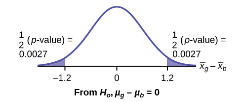
So, ${\overline{x}}_{g}-{\overline{x}}_{b}$ = 2 – 3.2 = –1.2
Half the p-value is below –1.2 and half is above 1.2.

Make a decision: Since α > p-value, reject H₀. This means you reject μ_g = μ_b. The means are different.

Press STAT. Arrow over to TESTS and press 4:2-SampTTest. Arrow over to Stats and press ENTER. Arrow down and enter 2 for the first sample mean, for Sx1, 9 for n1, 3.2 for the second sample mean, 1 for Sx2, and 16 for n2. Arrow down to μ1: and arrow to does not equal μ2. Press ENTER. Arrow down to Pooled: and No. Press ENTER. Arrow down to Calculate and press ENTER. The p-value is p = 0.0054, the dfs are approximately 18.8462, and the test statistic is -3.14. Do the procedure again but instead of Calculate do Draw.

Conclusion: At the 5% level of significance, the sample data show there is sufficient evidence to conclude that the mean number of hours that girls and boys aged seven to 11 play sports per day is different (mean number of hours boys aged seven to 11 play sports per day is greater than the mean number of hours played by girls OR the mean number of hours girls aged seven to 11 play sports per day is greater than the mean number of hours played by boys).

Try It

Two samples are shown in (Figure). Both have normal distributions. The means for the two populations are thought to be the same. Is there a difference in the means? Test at the 5% level of significance.

	Sample Size	Sample Mean	Sample Standard Deviation
Population A	25	5	1
Population B	16	4.7	1.2

NOTE

When the sum of the sample sizes is larger than 30 (n₁ + n₂ > 30) you can use the normal distribution to approximate the Student’s t.

A study is done by a community group in two neighboring colleges to determine which one graduates students with more math classes. College A samples 11 graduates. Their average is four math classes with a standard deviation of 1.5 math classes. College B samples nine graduates. Their average is 3.5 math classes with a standard deviation of one math class. The community group believes that a student who graduates from college A has taken more math classes, on the average. Both populations have a normal distribution. Test at a 1% significance level. Answer the following questions.

a. Is this a test of two means or two proportions?

a. two means

b. Are the populations standard deviations known or unknown?

b. unknown

c. Which distribution do you use to perform the test?

c. Student’s t

d. What is the random variable?

d. ${\overline{X}}_{A}-{\overline{X}}_{B}$

e. What are the null and alternate hypotheses? Write the null and alternate hypotheses in words and in symbols.

e.

${H}_{o}:{\mu }_{A}\le {\mu }_{B}$
${H}_{a}:{\mu }_{A}>{\mu }_{B}$

f. Is this test right-, left-, or two-tailed?

f.

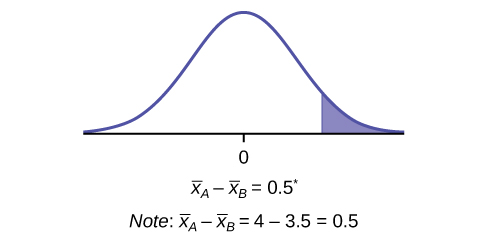
right

g. What is the p-value?

g. 0.1928

h. Do you reject or not reject the null hypothesis?

h. Do not reject.

i. Conclusion:

i. At the 1% level of significance, from the sample data, there is not sufficient evidence to conclude that a student who graduates from college A has taken more math classes, on the average, than a student who graduates from college B.

Try It

A study is done to determine if Company A retains its workers longer than Company B. Company A samples 15 workers, and their average time with the company is five years with a standard deviation of 1.2. Company B samples 20 workers, and their average time with the company is 4.5 years with a standard deviation of 0.8. The populations are normally distributed.

Are the population standard deviations known?
Conduct an appropriate hypothesis test. At the 5% significance level, what is your conclusion?

A professor at a large community college wanted to determine whether there is a difference in the means of final exam scores between students who took his statistics course online and the students who took his face-to-face statistics class. He believed that the mean of the final exam scores for the online class would be lower than that of the face-to-face class. Was the professor correct? The randomly selected 30 final exam scores from each group are listed in (Figure) and (Figure).

Online Class
67.6	41.2	85.3	55.9	82.4	91.2	73.5	94.1	64.7	64.7
70.6	38.2	61.8	88.2	70.6	58.8	91.2	73.5	82.4	35.5
94.1	88.2	64.7	55.9	88.2	97.1	85.3	61.8	79.4	79.4

Face-to-face Class
77.9	95.3	81.2	74.1	98.8	88.2	85.9	92.9	87.1	88.2
69.4	57.6	69.4	67.1	97.6	85.9	88.2	91.8	78.8	71.8
98.8	61.2	92.9	90.6	97.6	100	95.3	83.5	92.9	89.4

Is the mean of the Final Exam scores of the online class lower than the mean of the Final Exam scores of the face-to-face class? Test at a 5% significance level. Answer the following questions:

Is this a test of two means or two proportions?
Are the population standard deviations known or unknown?
Which distribution do you use to perform the test?
What is the random variable?
What are the null and alternative hypotheses? Write the null and alternative hypotheses in words and in symbols.
Is this test right, left, or two tailed?
What is the p-value?
Do you reject or not reject the null hypothesis?
At the ___ level of significance, from the sample data, there ______ (is/is not) sufficient evidence to conclude that ______.

two means
unknown
Student’s t
1. H₀: μ₁ = μ₂ Null hypothesis: the means of the final exam scores are equal for the online and face-to-face statistics classes.
2. H_a: μ₁ < μ₂ Alternative hypothesis: the mean of the final exam scores of the online class is less than the mean of the final exam scores of the face-to-face class.
left-tailed
p-value = 0.0011
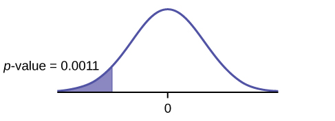
Reject the null hypothesis
The professor was correct. The evidence shows that the mean of the final exam scores for the online class is lower than that of the face-to-face class.
At the 5% level of significance, from the sample data, there is (is/is not) sufficient evidence to conclude that the mean of the final exam scores for the online class is less than the mean of final exam scores of the face-to-face class.

Cohen’s Standards for Small, Medium, and Large Effect SizesCohen’s d is a measure of effect size based on the differences between two means. Cohen’s d, named for United States statistician Jacob Cohen, measures the relative strength of the differences between the means of two populations based on sample data. The calculated value of effect size is then compared to Cohen’s standards of small, medium, and large effect sizes.

Cohen’s Standard Effect Sizes
Size of effect	d
Small	0.2
medium	0.5
Large	0.8

Cohen’s d is the measure of the difference between two means divided by the pooled standard deviation: $d=\frac{{\overline{x}}_{1}-{\overline{x}}_{2}}{{s}_{pooled}}$ where ${s}_{pooled}=\sqrt{\frac{\left({n}_{1}-1\right){s}_{1}^{2}+\left({n}_{2}-1\right){s}_{2}^{2}}{{n}_{1}+{n}_{2}-2}}$

Calculate Cohen’s d for (Figure). Is the size of the effect small, medium, or large? Explain what the size of the effect means for this problem.

μ₁ = 4 s₁ = 1.5 n₁ = 11
μ₂ = 3.5 s₂ = 1 n₂ = 9
d = 0.384
The effect is small because 0.384 is between Cohen’s value of 0.2 for small effect size and 0.5 for medium effect size. The size of the differences of the means for the two colleges is small indicating that there is not a significant difference between them.

Calculate Cohen’s d for (Figure). Is the size of the effect small, medium or large? Explain what the size of the effect means for this problem.

d = 0.834; Large, because 0.834 is greater than Cohen’s 0.8 for a large effect size. The size of the differences between the means of the Final Exam scores of online students and students in a face-to-face class is large indicating a significant difference.

Try It

Weighted alpha is a measure of risk-adjusted performance of stocks over a period of a year. A high positive weighted alpha signifies a stock whose price has risen while a small positive weighted alpha indicates an unchanged stock price during the time period. Weighted alpha is used to identify companies with strong upward or downward trends. The weighted alpha for the top 30 stocks of banks in the northeast and in the west as identified by Nasdaq on May 24, 2013 are listed in (Figure) and (Figure), respectively.

Northeast
94.2	75.2	69.6	52.0	48.0	41.9	36.4	33.4	31.5	27.6
77.3	71.9	67.5	50.6	46.2	38.4	35.2	33.0	28.7	26.5
76.3	71.7	56.3	48.7	43.2	37.6	33.7	31.8	28.5	26.0

West
126.0	70.6	65.2	51.4	45.5	37.0	33.0	29.6	23.7	22.6
116.1	70.6	58.2	51.2	43.2	36.0	31.4	28.7	23.5	21.6
78.2	68.2	55.6	50.3	39.0	34.1	31.0	25.3	23.4	21.5

Is there a difference in the weighted alpha of the top 30 stocks of banks in the northeast and in the west? Test at a 5% significance level. Answer the following questions:

Is this a test of two means or two proportions?
Are the population standard deviations known or unknown?
Which distribution do you use to perform the test?
What is the random variable?
What are the null and alternative hypotheses? Write the null and alternative hypotheses in words and in symbols.
Is this test right, left, or two tailed?
What is the p-value?
Do you reject or not reject the null hypothesis?
At the ___ level of significance, from the sample data, there ______ (is/is not) sufficient evidence to conclude that ______.
Calculate Cohen’s d and interpret it.

Use the following information to answer the next 15 exercises: Indicate if the hypothesis test is for

independent group means, population standard deviations, and/or variances known
independent group means, population standard deviations, and/or variances unknown
matched or paired samples
single mean
two proportions
single proportion

It is believed that 70% of males pass their drivers test in the first attempt, while 65% of females pass the test in the first attempt. Of interest is whether the proportions are in fact equal.

two proportions

A new laundry detergent is tested on consumers. Of interest is the proportion of consumers who prefer the new brand over the leading competitor. A study is done to test this.

A new windshield treatment claims to repel water more effectively. Ten windshields are tested by simulating rain without the new treatment. The same windshields are then treated, and the experiment is run again. A hypothesis test is conducted.

matched or paired samples

The known standard deviation in salary for all mid-level professionals in the financial industry is $11,000. Company A and Company B are in the financial industry. Suppose samples are taken of mid-level professionals from Company A and from Company B. The sample mean salary for mid-level professionals in Company A is $80,000. The sample mean salary for mid-level professionals in Company B is $96,000. Company A and Company B management want to know if their mid-level professionals are paid differently, on average.

The average worker in Germany gets eight weeks of paid vacation.

single mean

According to a television commercial, 80% of dentists agree that Ultrafresh toothpaste is the best on the market.

It is believed that the average grade on an English essay in a particular school system for females is higher than for males. A random sample of 31 females had a mean score of 82 with a standard deviation of three, and a random sample of 25 males had a mean score of 76 with a standard deviation of four.

independent group means, population standard deviations and/or variances unknown

The league mean batting average is 0.280 with a known standard deviation of 0.06. The Rattlers and the Vikings belong to the league. The mean batting average for a sample of eight Rattlers is 0.210, and the mean batting average for a sample of eight Vikings is 0.260. There are 24 players on the Rattlers and 19 players on the Vikings. Are the batting averages of the Rattlers and Vikings statistically different?

In a random sample of 100 forests in the United States, 56 were coniferous or contained conifers. In a random sample of 80 forests in Mexico, 40 were coniferous or contained conifers. Is the proportion of conifers in the United States statistically more than the proportion of conifers in Mexico?

two proportions

A new medicine is said to help improve sleep. Eight subjects are picked at random and given the medicine. The means hours slept for each person were recorded before starting the medication and after.

It is thought that teenagers sleep more than adults on average. A study is done to verify this. A sample of 16 teenagers has a mean of 8.9 hours slept and a standard deviation of 1.2. A sample of 12 adults has a mean of 6.9 hours slept and a standard deviation of 0.6.

independent group means, population standard deviations and/or variances unknown

Varsity athletes practice five times a week, on average.

A sample of 12 in-state graduate school programs at school A has a mean tuition of $64,000 with a standard deviation of $8,000. At school B, a sample of 16 in-state graduate programs has a mean of $80,000 with a standard deviation of $6,000. On average, are the mean tuitions different?

independent group means, population standard deviations and/or variances unknown

A new WiFi range booster is being offered to consumers. A researcher tests the native range of 12 different routers under the same conditions. The ranges are recorded. Then the researcher uses the new WiFi range booster and records the new ranges. Does the new WiFi range booster do a better job?

A high school principal claims that 30% of student athletes drive themselves to school, while 4% of non-athletes drive themselves to school. In a sample of 20 student athletes, 45% drive themselves to school. In a sample of 35 non-athlete students, 6% drive themselves to school. Is the percent of student athletes who drive themselves to school more than the percent of nonathletes?

two proportions

Use the following information to answer the next three exercises: A study is done to determine which of two soft drinks has more sugar. There are 13 cans of Beverage A in a sample and six cans of Beverage B. The mean amount of sugar in Beverage A is 36 grams with a standard deviation of 0.6 grams. The mean amount of sugar in Beverage B is 38 grams with a standard deviation of 0.8 grams. The researchers believe that Beverage B has more sugar than Beverage A, on average. Both populations have normal distributions.

Are standard deviations known or unknown?

What is the random variable?

The random variable is the difference between the mean amounts of sugar in the two soft drinks.

Is this a one-tailed or two-tailed test?

Use the following information to answer the next 12 exercises: The U.S. Center for Disease Control reports that the mean life expectancy was 47.6 years for whites born in 1900 and 33.0 years for nonwhites. Suppose that you randomly survey death records for people born in 1900 in a certain county. Of the 124 whites, the mean life span was 45.3 years with a standard deviation of 12.7 years. Of the 82 nonwhites, the mean life span was 34.1 years with a standard deviation of 15.6 years. Conduct a hypothesis test to see if the mean life spans in the county were the same for whites and nonwhites.

Is this a test of means or proportions?

means

State the null and alternative hypotheses.

H₀: __________
H_a: __________

Is this a right-tailed, left-tailed, or two-tailed test?

two-tailed

In symbols, what is the random variable of interest for this test?

In words, define the random variable of interest for this test.

the difference between the mean life spans of whites and nonwhites

Which distribution (normal or Student’s t) would you use for this hypothesis test?

Explain why you chose the distribution you did for (Figure).

This is a comparison of two population means with unknown population standard deviations.

Calculate the test statistic and p-value.

Sketch a graph of the situation. Label the horizontal axis. Mark the hypothesized difference and the sample difference. Shade the area corresponding to the p-value.

Check student’s solution.

Find the p-value.

At a pre-conceived α = 0.05, what is your:

Decision:
Reason for the decision:
Conclusion (write out in a complete sentence):

Reject the null hypothesis
p-value < 0.05
There is not enough evidence at the 5% level of significance to support the claim that life expectancy in the 1900s is different between whites and nonwhites.

Does it appear that the means are the same? Why or why not?

Homework

DIRECTIONS: For each of the word problems, use a solution sheet to do the hypothesis test. The solution sheet is found in Appendix E. Please feel free to make copies of the solution sheets. For the online version of the book, it is suggested that you copy the .doc or the .pdf files.

NOTE

If you are using a Student’s t-distribution for a homework problem in what follows, including for paired data, you may assume that the underlying population is normally distributed. (When using these tests in a real situation, you must first prove that assumption, however.)

The mean number of English courses taken in a two–year time period by male and female college students is believed to be about the same. An experiment is conducted and data are collected from 29 males and 16 females. The males took an average of three English courses with a standard deviation of 0.8. The females took an average of four English courses with a standard deviation of 1.0. Are the means statistically the same?

A student at a four-year college claims that mean enrollment at four–year colleges is higher than at two–year colleges in the United States. Two surveys are conducted. Of the 35 two–year colleges surveyed, the mean enrollment was 5,068 with a standard deviation of 4,777. Of the 35 four-year colleges surveyed, the mean enrollment was 5,466 with a standard deviation of 8,191.

Subscripts: 1: two-year colleges; 2: four-year colleges

H₀: μ₁ ≥ μ₂
H_a: μ₁ < μ₂
${\overline{X}}_{1}-{\overline{X}}_{2}$ is the difference between the mean enrollments of the two-year colleges and the four-year colleges.
Student’s-t
test statistic: -0.2480
p-value: 0.4019
Check student’s solution.
1. Alpha: 0.05
2. Decision: Do not reject
3. Reason for Decision: p-value > alpha
4. Conclusion: At the 5% significance level, there is sufficient evidence to conclude that the mean enrollment at four-year colleges is higher than at two-year colleges.

At Rachel’s 11^th birthday party, eight girls were timed to see how long (in seconds) they could hold their breath in a relaxed position. After a two-minute rest, they timed themselves while jumping. The girls thought that the mean difference between their jumping and relaxed times would be zero. Test their hypothesis.

Relaxed time (seconds)	Jumping time (seconds)
26	21
47	40
30	28
22	21
23	25
45	43
37	35
29	32

Mean entry-level salaries for college graduates with mechanical engineering degrees and electrical engineering degrees are believed to be approximately the same. A recruiting office thinks that the mean mechanical engineering salary is actually lower than the mean electrical engineering salary. The recruiting office randomly surveys 50 entry level mechanical engineers and 60 entry level electrical engineers. Their mean salaries were $46,100 and $46,700, respectively. Their standard deviations were $3,450 and $4,210, respectively. Conduct a hypothesis test to determine if you agree that the mean entry-level mechanical engineering salary is lower than the mean entry-level electrical engineering salary.

Subscripts: 1: mechanical engineering; 2: electrical engineering

H₀: µ₁ ≥ µ₂
H_a: µ₁ < µ₂
${\overline{X}}_{1}-{\overline{X}}_{2}$ is the difference between the mean entry level salaries of mechanical engineers and electrical engineers.
t₁₀₈
test statistic: t = –0.82
p-value: 0.2061
Check student’s solution.
1. Alpha: 0.05
2. Decision: Do not reject the null hypothesis.
3. Reason for Decision: p-value > alpha
4. Conclusion: At the 5% significance level, there is insufficient evidence to conclude that the mean entry-level salaries of mechanical engineers is lower than that of electrical engineers.

Marketing companies have collected data implying that teenage girls use more ring tones on their cellular phones than teenage boys do. In one particular study of 40 randomly chosen teenage girls and boys (20 of each) with cellular phones, the mean number of ring tones for the girls was 3.2 with a standard deviation of 1.5. The mean for the boys was 1.7 with a standard deviation of 0.8. Conduct a hypothesis test to determine if the means are approximately the same or if the girls’ mean is higher than the boys’ mean.

Use the information from (Figure) to answer the next four exercises.

Using the data from Lap 1 only, conduct a hypothesis test to determine if the mean time for completing a lap in races is the same as it is in practices.

H₀: µ₁ = µ₂
H_a: µ₁ ≠ µ₂
${\overline{X}}_{1}-{\overline{X}}_{2}$ is the difference between the mean times for completing a lap in races and in practices.
t_20.32
test statistic: –4.70
p-value: 0.0001
Check student’s solution.
1. Alpha: 0.05
2. Decision: Reject the null hypothesis.
3. Reason for Decision: p-value < alpha
4. Conclusion: At the 5% significance level, there is sufficient evidence to conclude that the mean time for completing a lap in races is different from that in practices.

Repeat the test in Exercise 10.83, but use Lap 5 data this time.

Repeat the test in Exercise 10.83, but this time combine the data from Laps 1 and 5.

H₀: µ₁ = µ₂
H_a: µ₁ ≠ µ₂
is the difference between the mean times for completing a lap in races and in practices.
t_40.94
test statistic: –5.08
p-value: zero
Check student’s solution.
1. Alpha: 0.05
2. Decision: Reject the null hypothesis.
3. Reason for Decision: p-value < alpha
4. Conclusion: At the 5% significance level, there is sufficient evidence to conclude that the mean time for completing a lap in races is different from that in practices.

In two to three complete sentences, explain in detail how you might use Terri Vogel’s data to answer the following question. “Does Terri Vogel drive faster in races than she does in practices?”

Use the following information to answer the next two exercises. The Eastern and Western Major League Soccer conferences have a new Reserve Division that allows new players to develop their skills. Data for a randomly picked date showed the following annual goals.

Western	Eastern
Los Angeles 9	D.C. United 9
FC Dallas 3	Chicago 8
Chivas USA 4	Columbus 7
Real Salt Lake 3	New England 6
Colorado 4	MetroStars 5
San Jose 4	Kansas City 3

Conduct a hypothesis test to answer the next two exercises.

The exact distribution for the hypothesis test is:

the normal distribution
the Student’s t-distribution
the uniform distribution
the exponential distribution

If the level of significance is 0.05, the conclusion is:

There is sufficient evidence to conclude that the W Division teams score fewer goals, on average, than the E teams
There is insufficient evidence to conclude that the W Division teams score more goals, on average, than the E teams.
There is insufficient evidence to conclude that the W teams score fewer goals, on average, than the E teams score.
Unable to determine

c

Suppose a statistics instructor believes that there is no significant difference between the mean class scores of statistics day students on Exam 2 and statistics night students on Exam 2. She takes random samples from each of the populations. The mean and standard deviation for 35 statistics day students were 75.86 and 16.91. The mean and standard deviation for 37 statistics night students were 75.41 and 19.73. The “day” subscript refers to the statistics day students. The “night” subscript refers to the statistics night students. A concluding statement is:

There is sufficient evidence to conclude that statistics night students’ mean on Exam 2 is better than the statistics day students’ mean on Exam 2.
There is insufficient evidence to conclude that the statistics day students’ mean on Exam 2 is better than the statistics night students’ mean on Exam 2.
There is insufficient evidence to conclude that there is a significant difference between the means of the statistics day students and night students on Exam 2.
There is sufficient evidence to conclude that there is a significant difference between the means of the statistics day students and night students on Exam 2.

Researchers interviewed street prostitutes in Canada and the United States. The mean age of the 100 Canadian prostitutes upon entering prostitution was 18 with a standard deviation of six. The mean age of the 130 United States prostitutes upon entering prostitution was 20 with a standard deviation of eight. Is the mean age of entering prostitution in Canada lower than the mean age in the United States? Test at a 1% significance level.

Test: two independent sample means, population standard deviations unknown.

Random variable: ${\overline{X}}_{1}-{\overline{X}}_{2}$

Distribution: H₀: μ₁ = μ₂H_a: μ₁ < μ₂ The mean age of entering prostitution in Canada is lower than the mean age in the United States.

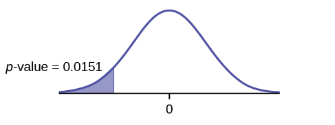
This is a normal distribution curve with mean equal to zero. A vertical line near the tail of the curve to the left of zero extends from the axis to the curve. The region under the curve to the left of the line is shaded representing p-value = 0.0157.

Graph: left-tailed

p-value : 0.0151

Decision: Do not reject H₀.

Conclusion: At the 1% level of significance, from the sample data, there is not sufficient evidence to conclude that the mean age of entering prostitution in Canada is lower than the mean age in the United States.

A powder diet is tested on 49 people, and a liquid diet is tested on 36 different people. Of interest is whether the liquid diet yields a higher mean weight loss than the powder diet. The powder diet group had a mean weight loss of 42 pounds with a standard deviation of 12 pounds. The liquid diet group had a mean weight loss of 45 pounds with a standard deviation of 14 pounds.

Suppose a statistics instructor believes that there is no significant difference between the mean class scores of statistics day students on Exam 2 and statistics night students on Exam 2. She takes random samples from each of the populations. The mean and standard deviation for 35 statistics day students were 75.86 and 16.91, respectively. The mean and standard deviation for 37 statistics night students were 75.41 and 19.73. The “day” subscript refers to the statistics day students. The “night” subscript refers to the statistics night students. An appropriate alternative hypothesis for the hypothesis test is:

μ_day > μ_night
μ_day < μ_night
μ_day = μ_night
μ_day ≠ μ_night

8.3 Inference for 2 Sample Proportion

1. A research study was conducted about gender differences in “sexting.” The researcher believed that the proportion of girls involved in “sexting” is less than the proportion of boys involved. The data collected in the spring of 2010 among a random sample of middle and high school students in a large school district in the southern United States is summarized below. Is the proportion of girls sending sexts less than the proportion of boys “sexting?” Test at a 1% level of significance.^[2]

Figure 8.26
	Males	Females
Sent “sexts”	183	156
Total number surveyed	2231	2169

This is a test of two population proportions. Let M and F be the subscripts for males and females. Then p_M and p_F are the desired population proportions.

Random variable: p̂_F − p̂_M = difference in the proportions of males and females who sent “sexts.”

H₀: p_F = p_M H₀: p_F – p_M = 0

H_a: p_F < p_M H_a: p_F – p_M < 0

The words “less than” tell you the test is left-tailed.

Distribution for the test: Since this is a test of two population proportions, the distribution is normal:

${p}_{p}=\frac{{x}_{F}+{x}_{M}}{{n}_{F}+{n}_{M}}=\frac{156+183}{2169+2231}=\text{0}\text{.077}$
$1-{p}_{p}=0.923$
Therefore,
${\hat{p}_{F}-\hat{p}_{M}\sim N\left(0,\sqrt{\left(0.077\right)\left(0.923\right)\left(\frac{1}{2169}+\frac{1}{2231}\right)}\right)$
p̂_F − p̂_M follows an approximate normal distribution.

Calculate the p-value using the normal distribution:
p-value = 0.1045
Estimated proportion for females: 0.0719
Estimated proportion for males: 0.082

Graph:

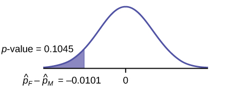
Decision: Since α < p-value, Do not reject H₀

Conclusion: At the 1% level of significance, from the sample data, there is not sufficient evidence to conclude that the proportion of girls sending “sexts” is less than the proportion of boys sending “sexts.”

Press STAT. Arrow over to TESTS and press 6:2-PropZTest. Arrow down and enter 156 for x1, 2169 for n1, 183 for x2, and 2231 for n2. Arrow down to p1: and arrow to less than p2. Press ENTER. Arrow down to Calculate and press ENTER. The p-value is P = 0.1045 and the test statistic is z = -1.256.

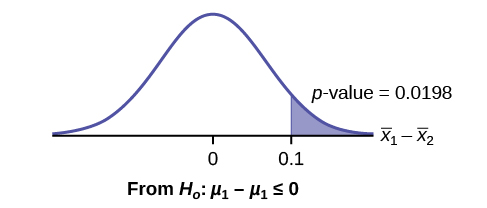
2. Researchers conducted a study of smartphone use among adults. A cell phone company claimed that iPhone smartphones are more popular with whites (non-Hispanic) than with African Americans. The results of the survey indicate that of the 232 African American cell phone owners randomly sampled, 5% have an iPhone. Of the 1,343 white cell phone owners randomly sampled, 10% own an iPhone. Test at the 5% level of significance. Is the proportion of white iPhone owners greater than the proportion of African American iPhone owners?^[3]

This is a test of two population proportions. Let W and A be the subscripts for the whites and African Americans. Then p_W and p_A are the desired population proportions.

Random variable: p̂_W − p̂_A = difference in the proportions of Android and iPhone users.

H₀: p_W = p_A H₀: p_W – p_A = 0

H_a: p_W > p_A H_a: p_W – p_A > 0

The words “more popular” indicate that the test is right-tailed.

Distribution for the test: The distribution is approximately normal:

${p}_{p}=\frac{{x}_{W}+{x}_{A}}{{n}_{W}+{n}_{A}}=\frac{134+12}{1343+232}=\text{ }0.0927$

$1-{p}_{p}=0.9073$

Therefore,

$\hat{p}_{W}-\hat{p}_{A}\backsim N\left(0,\sqrt{\left(0.0927\right)\left(0.9073\right)\left(\frac{1}{1343}+\frac{1}{232}\right)}\right)$

$\hat{p}_{W}-\hat{p}_{A}$ follows an approximate normal distribution.

Calculate the p-value using the normal distribution:
p-value = 0.0077
Estimated proportion for group A: 0.10
Estimated proportion for group B: 0.05

<!– LALALA ♪♫♪♫ CONTINUE INSERTING NEW EXAMPLE 3 HERE –>

Graph:

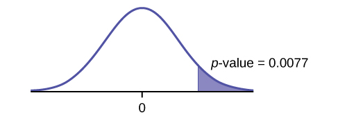
Decision: Since α > p-value, reject the H₀.

Conclusion: At the 5% level of significance, from the sample data, there is sufficient evidence to conclude that a larger proportion of white cell phone owners use iPhones than African Americans.

3. An interested citizen wanted to know if Democratic U. S. senators are older than Republican U.S. senators, on average. On May 26 2013, the mean age of 30 randomly selected Republican Senators was 61 years 247 days old (61.675 years) with a standard deviation of 10.17 years. The mean age of 30 randomly selected Democratic senators was 61 years 257 days old (61.704 years) with a standard deviation of 9.55 years.^[4]

Do the data indicate that Democratic senators are older than Republican senators, on average? Test at a 5% level of significance.

This is a test of two independent groups, two population means. The population standard deviations are unknown, but the sum of the sample sizes is 30 + 30 = 60, which is greater than 30, so we can use the normal approximation to the Student’s-t distribution. Subscripts: 1: Democratic senators 2: Republican senators

Random variable: ${\overline{X}}_{1}\text{ - }{\overline{X}}_{2}$ = difference in the mean age of Democratic and Republican U.S. senators.

H₀: µ₁ ≤ µ₂ H₀: µ₁ – µ₂ ≤ 0

H_a: µ₁ > µ₂ H_a: µ₁ – µ₂ > 0

The words “older than” translates as a “>” symbol and goes into H_a. Therefore, this is a right-tailed test.

Distribution for the test: The distribution is the normal approximation to the Student’s t for means, independent groups. Using the formula, the distribution is: ${\overline{X}}_{1}-{\overline{X}}_{2}\sim N\left[0,\sqrt{\frac{{\left(9.55\right)}^{2}}{30}+\frac{{\left(10.17\right)}^{2}}{30}}\right]$

Since µ₁ ≤ µ₂, µ₁ – µ₂ ≤ 0 and the mean for the normal distribution is zero.

(Calculating the p-value using the normal distribution givesp-value = 0.4955)

Graph:

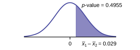
This is a normal distribution curve with mean equal to zero. A vertical line to the right of zero extends from the axis to the curve. The region under the curve to the right of the line is shaded representing p-value = 0.4955. — Figure 8.29

Compare α and the p-value:α = 0.05 and p-value = 0.4955. Therefore, α < p-value.

Make a decision: Since α < p-value, do not reject H₀.

Conclusion: At the 5% level of significance, from the sample data, there is not sufficient evidence to conclude that the mean age of Democratic senators is greater than the mean age of the Republican senators.

4. A concerned group of citizens wanted to know if the proportion of forcible rapes in Texas was different in 2011 than in 2010. Their research showed that of the 113,231 violent crimes in Texas in 2010, 7,622 of them were forcible rapes. In 2011, 7,439 of the 104,873 violent crimes were in the forcible rape category.^[5] Test at a 5% significance level. Answer the following questions:

a. Is this a test of two means or two proportions?

b. Which distribution do you use to perform the test?

c. What is the random variable?

d. What are the null and alternative hypothesis? Write the null and alternative hypothesis in symbols.

e. Is this test right-, left-, or two-tailed?

f. What is the p-value?

g. Do you reject or not reject the null hypothesis?

h. At the ___ level of significance, from the sample data, there ______ (is/is not) sufficient evidence to conclude that ____________.

5. Two types of phone operating system are being tested to determine if there is a difference in the proportions of system failures (crashes). Fifteen out of a random sample of 150 phones with OS₁ had system failures within the first eight hours of operation. Nine out of another random sample of 150 phones with OS₂ had system failures within the first eight hours of operation. OS₂ is believed to be more stable (have fewer crashes) than OS₁.

a. Is this a test of means or proportions?

b. What is the random variable?

$\hat{p}_{OS1} -\hat{p}_{OS2}$ = difference in the proportions of phones that had system failures within the first eight hours of operation with OS₁ and OS₂.

c. State the null and alternative hypotheses.

d. What is the p-value?

0.1018

e. What can you conclude about the two operating systems?

6. In the recent Census, three percent of the U.S. population reported being of two or more races. However, the percent varies tremendously from state to state. Suppose that two random surveys are conducted. In the first random survey, out of 1,000 North Dakotans, only nine people reported being of two or more races. In the second random survey, out of 500 Nevadans, 17 people reported being of two or more races.^[6] Conduct a hypothesis test to determine if the population percents are the same for the two states or if the percent for Nevada is statistically higher than for North Dakota.

a. Is this a test of means or proportions?

proportions

b. State the null and alternative hypotheses.

c. Is this a right-tailed, left-tailed, or two-tailed test? How do you know?

right-tailed

d. What is the random variable of interest for this test?

In words, define the random variable for this test.

e. The random variable is the difference in proportions (percents) of the populations that are of two or more races in Nevada and North Dakota.

f. Which distribution (normal or Student’s t) would you use for this hypothesis test?

g. Explain why you chose the distribution you did.

Our sample sizes are much greater than five each, so we use the normal for two proportions distribution for this hypothesis test.

h. Calculate the test statistic.

i. Sketch a graph of the situation. Mark the hypothesized difference and the sample difference. Shade the area corresponding to the p-value.

This is a horizontal axis with arrows at each end. The axis is labeled p'N - p'ND — Figure 8.30

j. Find the p-value.

k. At a pre-conceived α = 0.05, what is your:

Decision:
Reason for the decision:
Conclusion (write out in a complete sentence):

Reject the null hypothesis.
p-value < alpha
At the 5% significance level, there is sufficient evidence to conclude that the proportion (percent) of the population that is of two or more races in Nevada is statistically higher than that in North Dakota.

l. Does it appear that the proportion of Nevadans who are two or more races is higher than the proportion of North Dakotans? Why or why not?

7. DIRECTIONS: For each of the word problems, use a solution sheet to do the hypothesis test. The solution sheet is found in (Figure). Please feel free to make copies of the solution sheets. For the online version of the book, it is suggested that you copy the .doc or the .pdf files.

Note: If you are using a Student’s t-distribution for one of the following homework problems, including for paired data, you may assume that the underlying population is normally distributed. (In general, you must first prove that assumption, however.)

a. A recent drug survey showed an increase in the use of drugs and alcohol among local high school seniors as compared to the national percent. Suppose that a survey of 100 local seniors and 100 national seniors is conducted to see if the proportion of drug and alcohol use is higher locally than nationally. Locally, 65 seniors reported using drugs or alcohol within the past month, while 60 national seniors reported using them.

b. A study is done to determine if students in the California state university system take longer to graduate, on average, than students enrolled in private universities. One hundred students from both the California state university system and private universities are surveyed. Suppose that from years of research, it is known that the population standard deviations are 1.5811 years and 1 year, respectively. The following data are collected. The California state university system students took on average 4.5 years with a standard deviation of 0.8. The private university students took on average 4.1 years with a standard deviation of 0.3.

8. We are interested in whether the proportions of female suicide victims for ages 15 to 24 are the same for the whites and the blacks races in the United States. We randomly pick one year, 1992, to compare the races. The number of suicides estimated in the United States in 1992 for white females is 4,930. Five hundred eighty were aged 15 to 24. The estimate for black females is 330. Forty were aged 15 to 24.^[7] We will let female suicide victims be our population.

H₀: P_W = P_B
H_a: P_W ≠ P_B
The random variable is the difference in the proportions of white and black suicide victims, aged 15 to 24.
normal for two proportions
test statistic: –0.1944
p-value: 0.8458
Check student’s solution.
1. Alpha: 0.05
2. Decision: Reject the null hypothesis.
3. Reason for decision: p-value > alpha
4. Conclusion: At the 5% significance level, there is insufficient evidence to conclude that the proportions of white and black female suicide victims, aged 15 to 24, are different.

9. Elizabeth Mjelde, an art history professor, was interested in whether the value from the Golden Ratio formula, $\left(\frac{\text{larger + smaller dimension}}{\text{larger dimension}}\right)$ was the same in the Whitney Exhibit for works from 1900 to 1919 as for works from 1920 to 1942. Thirty-seven early works were sampled, averaging 1.74 with a standard deviation of 0.11. Sixty-five of the later works were sampled, averaging 1.746 with a standard deviation of 0.1064.^[8] Do you think that there is a significant difference in the Golden Ratio calculation?

10. A recent year was randomly picked from 1985 to the present. In that year, there were 2,051 Hispanic students at Cabrillo College out of a total of 12,328 students. At Lake Tahoe College, there were 321 Hispanic students out of a total of 2,441 students.^[9] In general, do you think that the percent of Hispanic students at the two colleges is basically the same or different?

Subscripts: 1 = Cabrillo College, 2 = Lake Tahoe College

H₀: p₁ = p₂
H_a: p₁ ≠ p₂
The random variable is the difference between the proportions of Hispanic students at Cabrillo College and Lake Tahoe College.
normal for two proportions
test statistic: 4.29
p-value: 0.00002
Check student’s solution.
1. Alpha: 0.05
2. Decision: Reject the null hypothesis.
3. Reason for decision: p-value < alpha
4. Conclusion: There is sufficient evidence to conclude that the proportions of Hispanic students at Cabrillo College and Lake Tahoe College are different.

11. Neuroinvasive West Nile virus is a severe disease that affects a person’s nervous system . It is spread by the Culex species of mosquito. In the United States in 2010 there were 629 reported cases of neuroinvasive West Nile virus out of a total of 1,021 reported cases and there were 486 neuroinvasive reported cases out of a total of 712 cases reported in 2011.^[10] Is the 2011 proportion of neuroinvasive West Nile virus cases more than the 2010 proportion of neuroinvasive West Nile virus cases? Using a 1% level of significance, conduct an appropriate hypothesis test.

“2011” subscript: 2011 group.
“2010” subscript: 2010 group

a. This is:

a test of two proportions
a test of two independent means
a test of a single mean
a test of matched pairs.

b. An appropriate null hypothesis is:

p₂₀₁₁ ≤ p₂₀₁₀
p₂₀₁₁ ≥ p₂₀₁₀
μ₂₀₁₁ ≤ μ₂₀₁₀
p₂₀₁₁ > p₂₀₁₀

Solution: a

c. The p-value is 0.0022. At a 1% level of significance, the appropriate conclusion is

There is sufficient evidence to conclude that the proportion of people in the United States in 2011 who contracted neuroinvasive West Nile disease is less than the proportion of people in the United States in 2010 who contracted neuroinvasive West Nile disease.
There is insufficient evidence to conclude that the proportion of people in the United States in 2011 who contracted neuroinvasive West Nile disease is more than the proportion of people in the United States in 2010 who contracted neuroinvasive West Nile disease.
There is insufficient evidence to conclude that the proportion of people in the United States in 2011 who contracted neuroinvasive West Nile disease is less than the proportion of people in the United States in 2010 who contracted neuroinvasive West Nile disease.
There is sufficient evidence to conclude that the proportion of people in the United States in 2011 who contracted neuroinvasive West Nile disease is more than the proportion of people in the United States in 2010 who contracted neuroinvasive West Nile disease.

12. Researchers conducted a study to find out if there is a difference in the use of eReaders by different age groups. Randomly selected participants were divided into two age groups. In the 16- to 29-year-old group, 7% of the 628 surveyed use eReaders, while 11% of the 2,309 participants 30 years old and older use eReaders.^[11]

Test: two independent sample proportions.

Random variable: p̂₁ – p̂₂

Distribution:
H₀: p₁ = p₂
H_a: p₁ ≠ p₂

The proportion of eReader users is different for the 16- to 29-year-old users from that of the 30 and older users.

Graph: two-tailed

p-value : 0.0033

Decision: Reject the null hypothesis.

Conclusion: At the 5% level of significance, from the sample data, there is sufficient evidence to conclude that the proportion of eReader users 16 to 29 years old is different from the proportion of eReader users 30 and older.

13. Adults aged 18 years old and older were randomly selected for a survey on obesity. Adults are considered obese if their body mass index (BMI) is at least 30. The researchers wanted to determine if the proportion of women who are obese in the south is less than the proportion of southern men who are obese. The results are shown below.^[12] Test at the 1% level of significance.

Figure 8.32
	Number who are obese	Sample size
Men	42,769	155,525
Women	67,169	248,775

14. Two computer users were discussing tablet computers. At one point in time a higher proportion of people ages 16 to 29 use tablets than the proportion of people age 30 and older. The figure below details the number of tablet owners for each age group. Test at the 1% level of significance.

Figure 8.33
	16–29 year olds	30 years old and older
Own a Tablet	69	231
Sample Size	628	2,309

Test: two independent sample proportions

Random variable: p̂₁ – p̂₂

Distribution:

H₀: p₁ = p₂
H_a: p₁ > p₂

A higher proportion of tablet owners are aged 16 to 29 years old than are 30 years old and older.

Graph: right-tailed

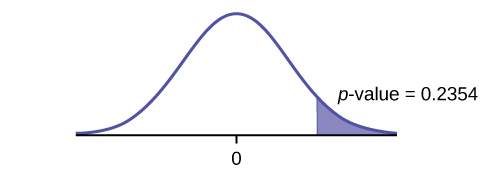
p-value: 0.2354

Decision: Do not reject the H₀.

Conclusion: At the 1% level of significance, from the sample data, there is not sufficient evidence to conclude that a higher proportion of tablet owners are aged 16 to 29 years old than are 30 years old and older.

15. A group of friends debated whether more men use smartphones than women. They consulted a research study of smartphone use among adults. The results of the survey indicate that of the 973 men randomly sampled, 379 use smartphones. For women, 404 of the 1,304 who were randomly sampled use smartphones.^[13] Test at the 5% level of significance.

16. While her husband spent 2½ hours picking out new speakers, a statistician decided to determine whether the percent of men who enjoy shopping for electronic equipment is higher than the percent of women who enjoy shopping for electronic equipment. The population was Saturday afternoon shoppers. Out of 67 men, 24 said they enjoyed the activity. Eight of the 24 women surveyed claimed to enjoy the activity. Interpret the results of the survey.

Subscripts: 1: men; 2: women

H₀: p₁ ≤ p₂
H_a: p₁ > p₂
p̂₁ – p̂₂ is the difference between the proportions of men and women who enjoy shopping for electronic equipment.
normal for two proportions
test statistic: 0.22
p-value: 0.4133
Check student’s solution.
1. Alpha: 0.05
2. Decision: Do not reject the null hypothesis.
3. Reason for Decision: p-value > alpha
4. Conclusion: At the 5% significance level, there is insufficient evidence to conclude that the proportion of men who enjoy shopping for electronic equipment is more than the proportion of women.

17. We are interested in whether children’s educational computer software costs less, on average, than children’s entertainment software. Thirty-six educational software titles were randomly picked from a catalog. The mean cost was $31.14 with a standard deviation of $4.69. Thirty-five entertainment software titles were randomly picked from the same catalog. The mean cost was $33.86 with a standard deviation of $10.87. Decide whether children’s educational software costs less, on average, than children’s entertainment software.

18. Joan Nguyen recently claimed that the proportion of college-age males with at least one pierced ear is as high as the proportion of college-age females. She conducted a survey in her classes. Out of 107 males, 20 had at least one pierced ear. Out of 92 females, 47 had at least one pierced ear. Do you believe that the proportion of males has reached the proportion of females?

H₀: p₁ = p₂
H_a: p₁ ≠ p₂
p̂₁ – p̂₂ is the difference between the proportions of men and women that have at least one pierced ear.
normal for two proportions
test statistic: –4.82
p-value: zero
Check student’s solution.
1. Alpha: 0.05
2. Decision: Reject the null hypothesis.
3. Reason for Decision: p-value < alpha
4. Conclusion: At the 5% significance level, there is sufficient evidence to conclude that the proportions of males and females with at least one pierced ear is different.

19. “To Breakfast or Not to Breakfast?” by Richard Ayore: In the American society, birthdays are one of those days that everyone looks forward to. People of different ages and peer groups gather to mark the 18th, 20th, …, birthdays. During this time, one looks back to see what he or she has achieved for the past year and also focuses ahead for more to come.

If, by any chance, I am invited to one of these parties, my experience is always different. Instead of dancing around with my friends while the music is booming, I get carried away by memories of my family back home in Kenya. I remember the good times I had with my brothers and sister while we did our daily routine.

Every morning, I remember we went to the shamba (garden) to weed our crops. I remember one day arguing with my brother as to why he always remained behind just to join us an hour later. In his defense, he said that he preferred waiting for breakfast before he came to weed. He said, “This is why I always work more hours than you guys!”

And so, to prove him wrong or right, we decided to give it a try. One day we went to work as usual without breakfast, and recorded the time we could work before getting tired and stopping. On the next day, we all ate breakfast before going to work. We recorded how long we worked again before getting tired and stopping. Of interest was our mean increase in work time. Though not sure, my brother insisted that it was more than two hours. Using the data below solve our problem.

Figure 8.35
Work hours with breakfast	Work hours without breakfast
8	6
7	5
9	5
5	4
9	7
8	7
10	7
7	5
6	6
9	5

H₀: µ_d = 0
H_a: µ_d > 0
The random variable X_d is the mean difference in work times on days when eating breakfast and on days when not eating breakfast.
t₉
test statistic: 4.8963
p-value: 0.0004
Check student’s solution.
1. Alpha: 0.05
2. Decision: Reject the null hypothesis.
3. Reason for Decision: p-value < alpha
4. Conclusion: At the 5% level of significance, there is sufficient evidence to conclude that the mean difference in work times on days when eating breakfast and on days when not eating breakfast has increased.

References

Image References

Figure 8.10: Figure 10.5.3 from LibreTexts Introductory Statistics (2020) (CC BY 4.0). Retrieved from https://stats.libretexts.org/Bookshelves/Introductory_Statistics/Book%3A_Introductory_Statistics_(OpenStax)/10%3A_Hypothesis_Testing_with_Two_Samples/10.05%3A_Matched_or_Paired_Samples

Figure 8.14: Figure 10.19 from OpenStax Introductory Statistics (2013) (CC BY 4.0). Retrieved from https://openstax.org/books/statistics/pages/10-solutions#fs-idm5499280-solution

Figure 8.19: Figure 10.23 from OpenStax Introductory Statistics (2013) (CC BY 4.0). Retrieved from https://openstax.org/books/statistics/pages/10-solutions#fs-idm5499280-solution

Figure 8.22: Figure 10.24 from OpenStax Introductory Statistics (2013) (CC BY 4.0). Retrieved from https://openstax.org/books/statistics/pages/10-solutions#fs-idm5499280-solution

Figure 8.27: Figure 10.8 from OpenStax Introductory Statistics (2013) (CC BY 4.0). Retrieved from https://openstax.org/books/introductory-statistics/pages/10-3-comparing-two-independent-population-proportions

Figure 8.28: Figure 10.9 from OpenStax Introductory Statistics (2013) (CC BY 4.0). Retrieved from https://openstax.org/books/introductory-statistics/pages/10-3-comparing-two-independent-population-proportions

Figure 8.29: Figure 10.6 from OpenStax Introductory Statistics (2013) (CC BY 4.0). Retrieved from https://openstax.org/books/introductory-statistics/pages/10-2-two-population-means-with-known-standard-deviations

Figure 8.30: Figure 10.17 from OpenStax Introductory Statistics (2013) (CC BY 4.0). Retrieved from https://openstax.org/books/statistics/pages/10-practice#element-814

Figure 8.31: Figure 10.21 from OpenStax Introductory Statistics (2013) (CC BY 4.0). Retrieved from https://openstax.org/books/statistics/pages/10-solutions

Figure 8.34: Figure 10.22 from OpenStax Introductory Statistics (2013) (CC BY 4.0). Retrieved from https://openstax.org/books/statistics/pages/10-solutions

Text

Data from Educational Resources, December catalog.

Data from Hilton Hotels. Available online at http://www.hilton.com (accessed June 17, 2013).

Data from Hyatt Hotels. Available online at http://hyatt.com (accessed June 17, 2013).

Data from Statistics, United States Department of Health and Human Services.

Data from Whitney Exhibit on loan to San Jose Museum of Art.

Data from the American Cancer Society. Available online at http://www.cancer.org/index (accessed June 17, 2013).

Data from the Chancellor’s Office, California Community Colleges, November 1994.

“State of the States.” Gallup, 2013. Available online at http://www.gallup.com/poll/125066/State-States.aspx?ref=interactive (accessed June 17, 2013).

“West Nile Virus.” Centers for Disease Control and Prevention. Available online at http://www.cdc.gov/ncidod/dvbid/westnile/index.htm (accessed June 17, 2013).

Data from the American Cancer Society. Available online at http://www.cancer.org/index (accessed June 17, 2013). ↵
Hinduja, Sameer. “Sexting Research and Gender Differences.” Cyberbulling Research Center, 2013. Available online at http://cyberbullying.us/blog/sexting-research-and-gender-differences/ (accessed June 17, 2013). ↵
“Smart Phone Users, By the Numbers.” Visually, 2013. Available online at http://visual.ly/smart-phone-users-numbers (accessed June 17, 2013). ↵
\“List of current United States Senators by Age.” Wikipedia. Available online at http://en.wikipedia.org/wiki/ List_of_current_United_States_Senators_by_age (accessed June 17, 2013). ↵
“Texas Crime Rates 1960–1012.” FBI, Uniform Crime Reports, 2013. Available online at: http://www.disastercenter.com/ crime/txcrime.htm (accessed June 17, 2013). ↵
“State of the States.” Gallup, 2013. Available online at http://www.gallup.com/poll/125066/StateStates.aspx?ref=interactive (accessed June 17, 2013). ↵
Data from Statistics, United States Department of Health and Human Services. ↵
Data from Whitney Exhibit on loan to San Jose Museum of Art ↵
Data from the Chancellor’s Office, California Community Colleges, November 1994. ↵
“West Nile Virus.” Centers for Disease Control and Prevention. Available online at http://www.cdc.gov/ncidod/dvbid/ westnile/index.htm (accessed June 17, 2013). ↵
Data from Educational Resources, December catalog. ↵
“State-Specific Prevalence of Obesity AmongAduls—Unites States, 2007.” MMWR, CDC. Available online at http://www.cdc.gov/mmwr/preview/mmwrhtml/mm5728a1.htm (accessed June 17, 2013). ↵
“Smart Phone Users, By the Numbers.” Visually, 2013. Available online at http://visual.ly/smart-phone-users-numbers (accessed June 17, 2013). ↵

License

Icon for the Creative Commons Attribution-ShareAlike 4.0 International License

Significant Statistics Copyright © 2020 by John Morgan Russell, OpenStaxCollege, OpenIntro is licensed under a Creative Commons Attribution-ShareAlike 4.0 International License, except where otherwise noted.

Starting cholesterol level	Ending cholesterol level
140	140
220	230
110	120
240	220
200	190
180	150
190	200
360	300
280	300
260	240

Starting cholesterol level	Ending cholesterol level
140	140
220	230
110	120
240	220
200	190
180	150
190	200
360	300
280	300
260	240

8.1 Inference for 2 Dependent Samples (Matched Pairs)

8.2 Inference for 2 Independent Sample Means

8.3 Inference for 2 Sample Proportions

8.1 Inference for 2 Dependent Samples (Matched Pairs)

8.2 Inference for 2 Independent Sample Means

8.3 Inference for 2 Sample Proportions

8.1 Inference for 2 Dependent Samples (Matched Pairs)

8.2 Inference for 2 Independent Sample Means

Homework

8.3 Inference for 2 Sample Proportion

Image References

Text

License

Share This Book

Starting cholesterol level	Ending cholesterol level
140	140
220	230
110	120
240	220
200	190
180	150
190	200
360	300
280	300
260	240