2.6 Measures of Center
Continuing through our acronym, SOCS, to describe the key aspects of our data:
- Shape
- Outliers
- Center
- Spread
The “center”, is a way of describing “central tendency” or “typical value” of a data set. The two most widely used measures of the “center” of the data are the mean (average) and the median. Most people are familiar with the ideas of these two; To calculate the mean weight of 50 people, add the 50 weights together and divide by 50. To find the median weight of the 50 people, order the data and find the number that splits the data into two equal parts.
However, some datasets may be better summarized by one or the other. The most “appropriate” measure of center depends on the shape of the distribution and presence of extreme values or potential outliers.
The Mean
The mean is the most common measure of the center. The words “mean” and “average” are often used interchangeably. The substitution of one word for the other is common practice. The technical term is “arithmetic mean” and “average” is technically a center location. However, in practice among non-statisticians, “average” is commonly accepted for “arithmetic mean.”
When each value in the data set is not unique, the mean can be calculated by multiplying each distinct value by its frequency and then dividing the sum by the total number of data values. The letter used to represent the sample mean is an x with a bar over it (pronounced “x bar”):  .
.
The Greek letter μ (pronounced “mew”) represents the population mean. One of the requirements for the sample mean to be a good estimate of the population mean is for the sample taken to be truly random. We will often use the sample mean to estimate the population mean.
Example
Calculate the mean of the sample: 1, 1, 1, 2, 2, 3, 4, 4, 4, 4, 4.
Your turn!
Calculate the mean of the sample: 7, 10, 14, 14, 15, 21, 38, 38, 38, 56.
The Median
The median is generally a better measure of the center when there are extreme values or outliers because it is more robust, or not affected by the precise numerical values of those outliers.
In many cases, especially for larger datasets you may choose to use the location function of the median rather than the traditional counting method.  .
.
Remember that this function simply tells you where to look for the median, not the actual value itself.
The letter n is the total number of data values in the sample. If n is an odd number, the median is the middle value of the ordered data (ordered smallest to largest). If n is an even number, the median is equal to the two middle values added together and divided by two after the data has been ordered.
For example, if the total number of data values is 97, then =  = 49. The median is the 49th value in the ordered data. If the total number of data values is 100, then
  . The median occurs midway between the 50th and 51st values. The location of the median and the value of the median are not the same. The upper case letter M is often used to represent the median. The next example illustrates the location of the median and the value of the median.
Example
AIDS data indicating the number of months a patient with AIDS lives after taking a new antibody drug are as follows (smallest to largest): 3, 4, 8, 8, 10, 11, 12, 13, 14, 15, 15, 16, 16, 17, 17, 18, 21, 22, 22, 24, 24, 25, 26, 26, 27, 27, 29, 29, 31, 32, 33, 33, 34, 34, 35, 37, 40, 44, 44, 47. Calculate the median.
Your turn!
Calculate the median of the sample: 7, 10, 14, 14, 15, 21, 38, 38, 38, 56.
The Mode
Another measure of the center is the mode. The mode is the most frequent value. There can be more than one mode in a data set as long as those values have the same frequency and that frequency is the highest. A data set with two modes is called bimodal. For example, five real estate exam scores are 430, 430, 480, 480, 495. The data set is bimodal because the scores 430 and 480 each occur twice.
When is the mode the best measure of the “center”? Consider a weight loss program that advertises a mean weight loss of six pounds the first week of the program. The mode might indicate that most people lose two pounds the first week, making the program less appealing.
- If we had the categorical data set {red, red, red, green, green, yellow, purple, black, blue} the mode is red. This is useful to us
- If we had the quantitative data set {1.0, 2.1, 2.1, 5.0, 5.1, 5.5, 5.7, 6.1, 6.2, 6.4, 6.6, 7.1, 7.8,8.1,8.9} the numerical mode is 2.1, but does not do a good job of telling us about the actual modality, or where the data is clustered.
Example
Statistics exam scores for 20 students are as follows:
50, 53, 59, 59, 63, 63, 72, 72, 72, 72, 72, 76, 78, 81, 83, 84, 84, 84, 90, 93
Find the mode.
Order Relationship of Measures of Center
Consider the following data set: 4, 5, 6, 6, 6, 7, 7, 7, 7, 7, 7, 8, 8, 8, 9, 10.
This data set can be represented by following histogram. Each interval has width one, and each value is located in the middle of an interval.
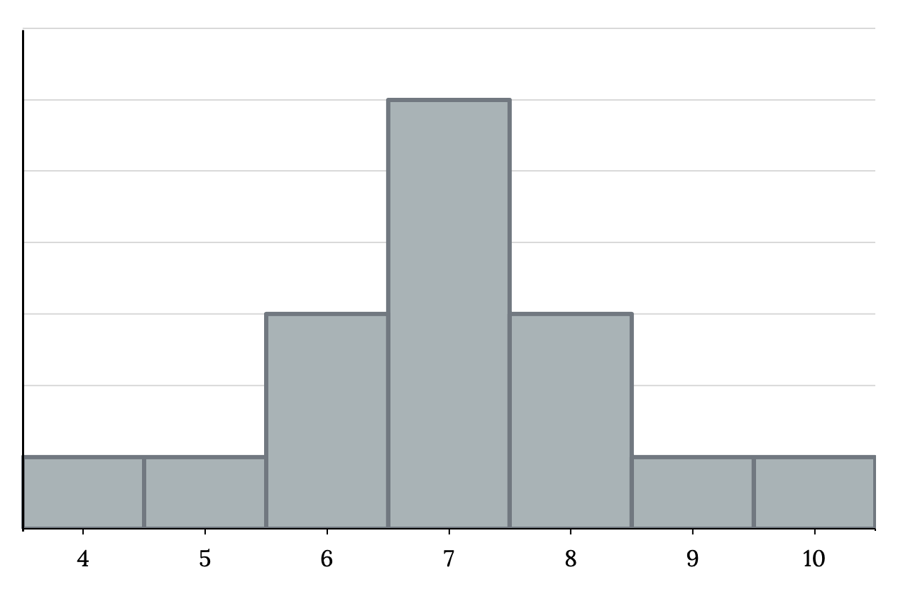
The histogram displays a symmetrical distribution of data. A distribution is symmetrical if a vertical line can be drawn at some point in the histogram such that the shape to the left and the right of the vertical line are mirror images of each other. The mean, the median, and the mode are each seven for these data. In a perfectly symmetrical distribution, the mean and the median are the same. This example has one mode (unimodal), and the mode is the same as the mean and median. In a symmetrical distribution that has two modes (bimodal), the two modes would be different from the mean and median.
The histogram for the data {4, 5, 6, 6, 6, 7, 7, 7, 7, 8} is not symmetrical. The right-hand side seems “chopped off” compared to the left side. A distribution of this type is called skewed to the left because it is pulled out to the left.
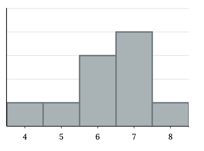
The mean is 6.3, the median is 6.5, and the mode is seven. Notice that the mean is less than the median, and they are both less than the mode. The mean and the median both reflect the skewing, but the mean reflects it more so.
The histogram for the data {6, 7, 7, 7, 7, 8, 8, 8, 9, 10} is also not symmetrical. It is skewed to the right.
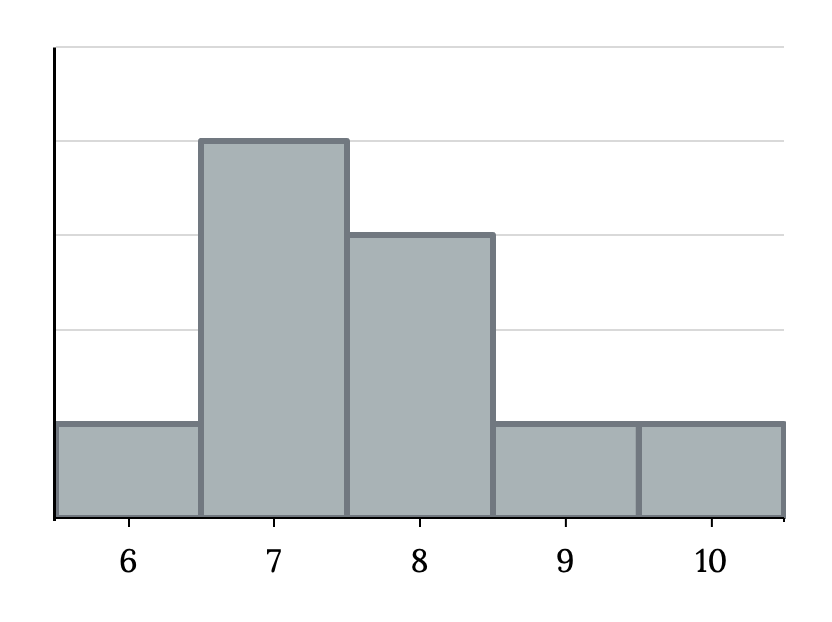
The mean is 7.7, the median is 7.5, and the mode is seven. Of the three statistics, the mean is the largest, while the mode is the smallest. Again, the mean reflects the skewing the most.
To summarize, generally if the distribution of data is skewed to the left, the mean is less than the median, which is often less than the mode. If the distribution of data is skewed to the right, the mode is often less than the median, which is less than the mean.
Skewness and symmetry become important when we discuss probability distributions in later chapters.
Example
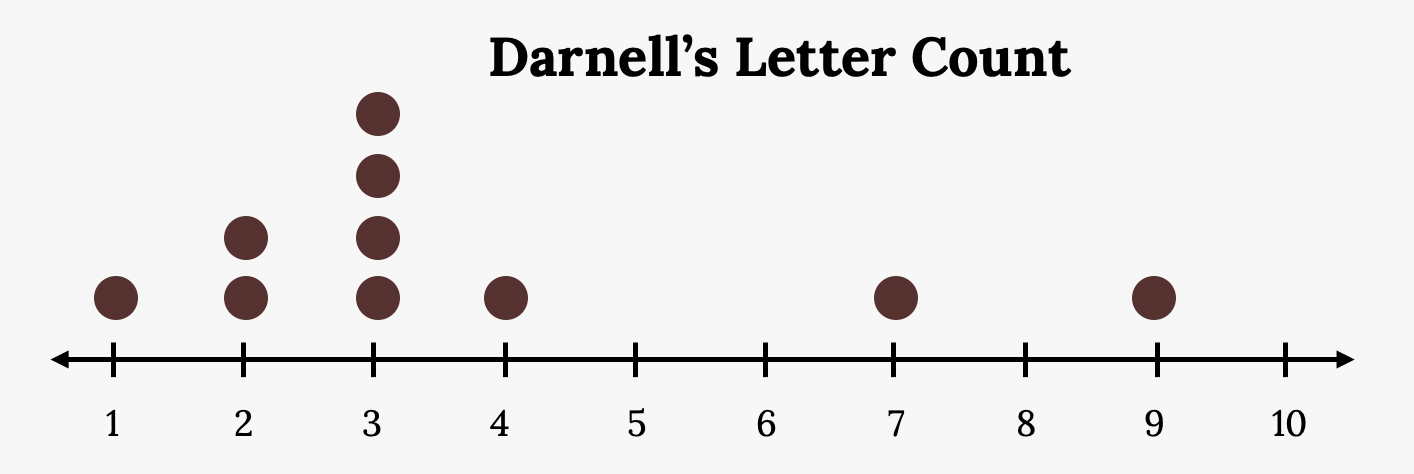
Statistics are used to compare and sometimes identify authors. The following lists shows a simple random sample that compares the letter counts for three authors.
Darnell: 7, 9, 3, 3, 3, 4, 1, 3, 2, 2
Mary: 3, 3, 3, 4, 1, 4, 3, 2, 3, 1
Lee: 2, 3, 4, 4, 4, 6, 6, 6, 8, 3
a. Make a dot plot for the three authors and compare the shapes.
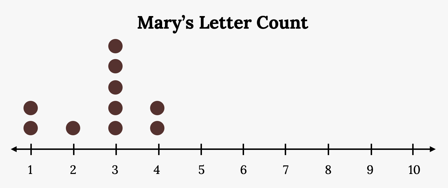
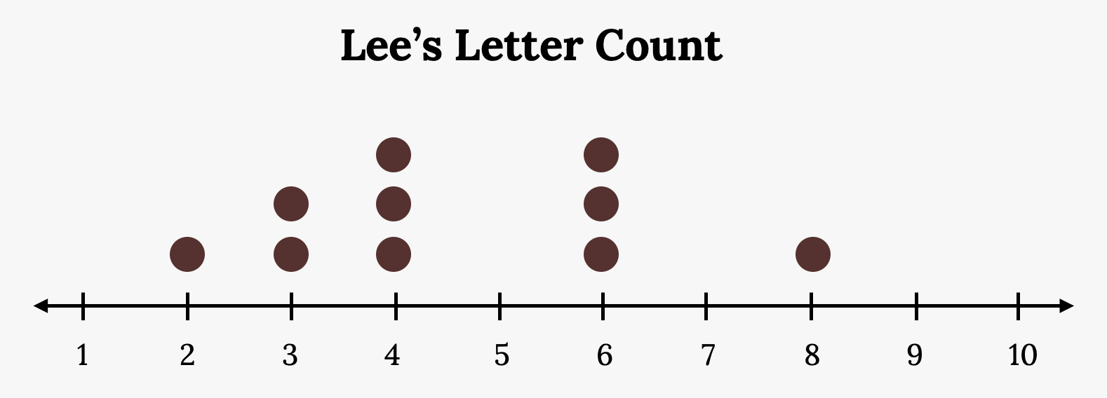
b. Calculate the mean for each.
c. Calculate the median for each.
d. Describe any pattern you notice between the shape and the measures of center.
Your Turn!
Suppose that in a small town of 50 people, one person earns $5,000,000 per year and the other 49 each earn $30,000. Which is the better measure of the “center”: the mean or the median?
Calculating the Mean of Grouped Frequency Tables
When only grouped data is available, you do not know the individual data values (we only know intervals and interval frequencies); therefore, you cannot compute an exact mean for the data set. What we must do is estimate the actual mean by calculating the mean of a frequency table. A frequency table is a data representation in which grouped data is displayed along with the corresponding frequencies. To calculate the mean from a grouped frequency table we can apply the basic definition of mean: mean =  We simply need to modify the definition to fit within the restrictions of a frequency table.
Since we do not know the individual data values we can instead find the midpoint of each interval. The midpoint is  . We can now modify the mean definition to be
  where f = the frequency of the interval and m = the midpoint of the interval.
Example
A frequency table displaying professor Blount’s last statistic test is shown.
- Find the best estimate of the class mean.
| Grade Interval | Number of Students |
|---|---|
| 50–56.5 | 1 |
| 56.5–62.5 | 0 |
| 62.5–68.5 | 4 |
| 68.5–74.5 | 4 |
| 74.5–80.5 | 2 |
| 80.5–86.5 | 3 |
| 86.5–92.5 | 4 |
| 92.5–98.5 | 1 |
Find the midpoints for all intervals
Calculate the sum of the product of each interval frequency.
Calculate the midpoint.
Your turn!
Maris conducted a study on the effect that playing video games has on memory recall. As part of her study, she compiled the following data:
| Hours Teenagers Spend on Video Games | Number of Teenagers |
|---|---|
| 0–3.5 | 3 |
| 3.5–7.5 | 7 |
| 7.5–11.5 | 12 |
| 11.5–15.5 | 7 |
| 15.5–19.5 | 9 |
What is the best estimate for the mean number of hours spent playing video games?
Image References
Figure 2.42: Kindred Grey (2020). “Figure 2.42.” CC BY-SA 4.0. Retrieved from https://commons.wikimedia.org/wiki/File:Figure_2.42.png
Figure 2.43: Kindred Grey (2020). “Figure 2.43.” CC BY-SA 4.0. Retrieved from https://commons.wikimedia.org/wiki/File:Figure_2.43.png
Figure 2.44: Kindred Grey (2020). “Figure 2.44.” CC BY-SA 4.0. Retrieved from https://commons.wikimedia.org/wiki/File:Figure_2.44.png
Figure 2.45: Kindred Grey via Virginia Tech (2020). “Figure 2.45” CC BY-SA 4.0. Retrieved from https://commons.wikimedia.org/wiki/File:Figure_2.45.png . Adaptation of Figure 2.21 from OpenStax Introductory Statistics (2013) (CC BY 4.0). Retrieved from https://openstax.org/books/statistics/pages/2-6-skewness-and-the-mean-median-and-mode
Figure 2.46: Kindred Grey via Virginia Tech (2020). “Figure 2.46” CC BY-SA 4.0. Retrieved from https://commons.wikimedia.org/wiki/File:Figure_2.46.png . Adaptation of Figure 2.22 from OpenStax Introductory Statistics (2013) (CC BY 4.0). Retrieved from https://openstax.org/books/statistics/pages/2-6-skewness-and-the-mean-median-and-mode
Figure 2.47: Kindred Grey via Virginia Tech (2020). “Figure 2.47” CC BY-SA 4.0. Retrieved from https://commons.wikimedia.org/wiki/File:Figure_2.47.png . Adaptation of Figure 2.23 from OpenStax Introductory Statistics (2013) (CC BY 4.0). Retrieved from https://openstax.org/books/statistics/pages/2-6-skewness-and-the-mean-median-and-mode
A number that measures the central tendency of the data
The middle number in a sorted list
The arithmetic mean, or average of a dataset
The arithmetic mean, or average of a population
Not affected by violations of assumptions such as outliers
The most frequently occurring value
How many peaks or clusters there appear to be in a quantitative distribution
