3.3 Compound Events
Recall the different combinations of relationships between two events:
| Independent? | |||
| Yes | No | ||
| Disjoint? | Yes | 1* | 2 |
| No | 3 | 4 | |
We must always go into a problem assuming two events are not mutually exclusive or independent. This “default” starting point is illustrated by the 4th position in the table above. Depending on the information your are given and assumptions you are able to make, you may move potions on this grid. Where you fall on the grid will dictate how we apply the rules we will discuss in this section to find probabilities of compound events.
There are two types of compound events we may be interested in, Unions and Intersections, each with their own set of rules and assumptions.
*Note: You will rarely, if ever, find yourself in this case
Finding Probabilities of Unions
To find a union we will typically use the addition rule. Intuitively the idea is that if we are looking for the outcomes in either event A or Event B, we should be able to simply add up the probabilities of each outcome. However, two events being mutually exclusive has big implications on how we apply the addition rule.
For Two Mutually Exclusive Events
The idea is simple when events are mutually exclusive. Picture a Venn diagram of two mutually exclusive events.
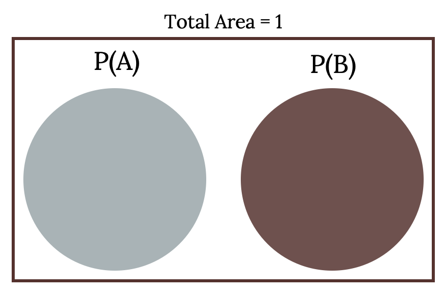
Not very exciting, but we need to note here that if A and B are mutually exclusive, then they have no shared outcomes. In other words no intersection exists between two disjoint events. In probability notation this means A ∩ B = Ø and P(A ∩ B) = 0.
In this case, the Union of A OR B is simply:
P(A ∪ B) = P(A) + P(B)
This is reflected in the previously mentioned Third Axiom of Probability (also called the disjoint addition rule).
Recall:
3. For each two events E1 and E2 with E1 ∩ E2 = Ø then P(E1 U E2) = P(E1) + P(E2)
Example
Klaus is trying to choose where to go on vacation. His two choices are: A = New Zealand and B = Alaska
- Klaus can only afford one vacation. The probability that he chooses A is P(A) = 0.6 and the probability that he chooses B is P(B) = 0.35.
- P(A AND B) = 0 because Klaus can only afford to take one vacation
- Therefore, the probability that he chooses either New Zealand or Alaska is P(A OR B) = P(A) + P(B) = 0.6 + 0.35 = 0.95.
- Note that the probability that he does not choose to go anywhere on vacation (the compliment) must then be 0.05.
For Two Non-Mutually Exclusive Events
When two events are not mutually exclusive it gets a bit trickier. Consider a Venn diagram of two non-mutually exclusive events.
![Two circles labaled P(A) and P(B) who do overlap in the middle [overlap labeled P(A and B)] whose total area = 1.](https://pressbooks.lib.vt.edu/app/uploads/sites/12/2020/12/3.12.png)
Here we can see that when A and B are not mutually exclusive, then they do have shared outcomes, or an intersection. If we try to apply the addition rule, we need to be careful not to double count those shared outcomes
If A and B are defined on a sample space, then: P(A ∪ B) = P(A) + P(B) – P(A ∩ B).
Example
Carlos plays college soccer. He makes a goal 65% of the time he shoots. Carlos is going to attempt two goals in a row in the next game. A = the event Carlos is successful on his first attempt. P(A) = 0.65. B = the event Carlos is successful on his second attempt. P(B) = 0.65. Carlos tends to shoot in streaks. The probability that he makes the second goal GIVEN that he made the first goal is 0.90.
a. Are A and B independent?
b. Are A and B mutually exclusive?
c. What is the probability that he makes both goals?
d. What is the probability that Carlos makes either the first goal or the second goal?
Your turn!
Felicity attends Reynolds CC in Richmond, VA. The probability that Felicity enrolls in a math class is 0.2 and the probability that she enrolls in a speech class is 0.65. The probability that she enrolls in a math class GIVEN that she enrolls in speech class is 0.25.
Let: M = math class, S = speech class, M|S = math given speech
a. Are M and S independent? Is P(M|S) = P(M)?
b. Are M and S mutually exclusive? Is P(M AND S) = 0?
c. What is the probability that Felicity enrolls in math and speech?
Find P(M AND S) = P(M|S)P(S).
d. What is the probability that Felicity enrolls in math or speech classes?
Find P(M OR S) = P(M) + P(S) – P(M AND S).
Applying the Addition Rule to Multiple Events
Let’s try to extend the ideas of the addition rule to more than two events. Again it will depend on whether these events are mutually exclusive or not.
More Than Two Mutually Exclusive Events
Let’s start by visualizing a Venn diagram of with 3 mutually exclusive events, A, B, and C. There would still be no intersections an we can simply apply the disjoint addition Rule resulting in:
P(A ∪ B ∪ C) = P(A) + P(B) + P(C)
Extending this beyond just three events follows easily. If they are mutually exclusive none of them have intersections and we should be able to apply our disjoint addition rule infinitely.
P(A ∪ B ∪ … ∪ N) = P(A) + P(B) + … + P(N)
As long as things are mutually exclusive we can just keep adding as many events we would like!
More Than Two Non-Mutually Exclusive Events
As with only two events things get a little bit trickier when we do have shared outcomes. Consider the Venn diagram below of three non-mutually exclusive events.
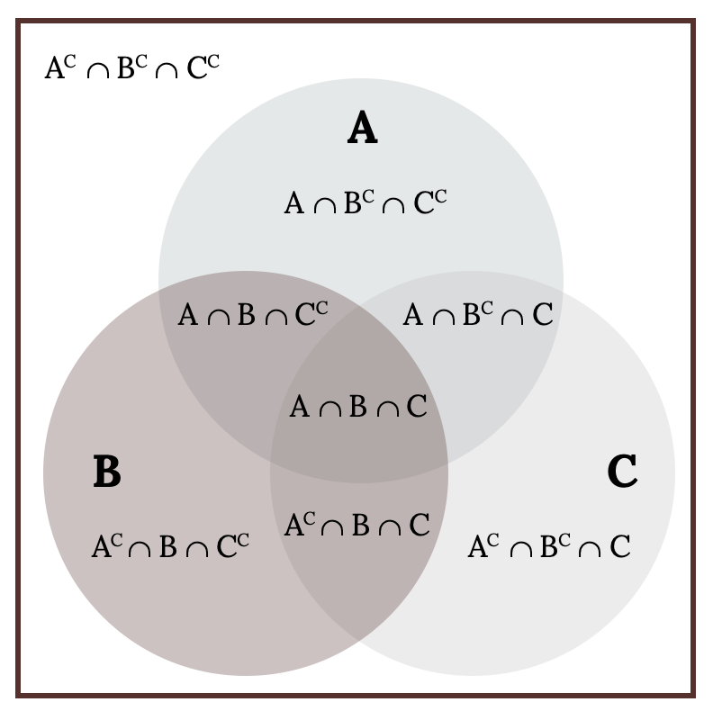
We have multiple double counting of intersections issues here. We could try subtracting the intersections as we did with two events, but that causes a new problem. If you subtract all three intersections once, you have now subtracted the triple intersection (A ∩ B ∩ C) three times thus not counting those outcomes at all! So after subtracting the three intersections to eliminate double counting we need to add back the triple intersection finally resulting in:
P(A ∪ B ∪ C) = P(A) + P(B) + P(C) – P(A ∩ B) – P(A ∩ C) – P(B ∩ C) + P(A ∩ B ∩ C)
Imagine extending this beyond 3 events! It’s a bit messy and changes slightly based on whether we have an odd or even number of events but is certainly doable if we are meticulous.
Finding Probabilities of Intersections
Let’s review a couple methods we have already seen that will help us find the intersection of two events:
- If two events are mutually exclusive we have already established they have no intersection i.e. P(A ∩ B) = 0.
- If we are given the right pieces we could even rearrange the addition rule as: P(A∩B) = P(B)+P(A) – P(A∪B)
Beyond these to find the probability of an intersection we can use the multiplication rule:
P(A ∩ B) = P(A)P(B|A) = P(B)P(A|B)
Notice we now have conditional probabilities involved and two different forms of the rule.
Finding a Conditional Probability
One way we can come up with conditional probabilities is to rewrite the multiplication rule as:
P(A|B) = 
(Notice what you are given goes in the denominator)
However, if we do not know the probability of the intersection this can leave us in a loop. In many cases we may just need to think carefully about a situation to come up with these conditional probabilities to apply our multiplication rule.
Conditional Probabilities for Two Independent Events
We now need to consider the implications of independence on conditional probabilities. Recall two independent events are events that have no effect on each other.
First, consider two dependent events: Let P(O) be the probability you oversleep and P(B) be the probability you eat breakfast. Oversleeping will likely have an effect on the probability you eat breakfast that morning so P(B|O) is of interest.
Now consider two independent events: Let P(G) be the probability you have green eyes and P(B) the probability you eat breakfast. Your eye color has no effect on whether you will eat breakfast or not, therefore P(B|G) is simply the same as P(B).
The Multiplication Rule for Two Independent Events
Now let’s think about the implications that independence then has on the multiplication rule. If A and B are independent then:
P(A|B) = P(A). So the multiplication rule, P(A ∩ B) = P(A|B)P(B) becomes P(A ∩ B) = P(A)P(B).
If two events are independent conditional probabilities are eliminated from the multiplication rule and things become much simpler
Showing Independence of Two Events
- Knowing what we now know about the implications of Independence on conditional probabilities and the multiplication rule, we can establish the following conditions. Events A and B are independent if one of the following is true:
- P(A|B) = P(A)
- P(B|A) = P(B)
- P(A AND B) = P(A)P(B)
Note that we only have to show one, all of these conditions are equivalent and imply each other.
Applying the Multiplication Rule to Multiple Events
Now we’ll extend the ideas of the multiplication rule to more than two events. How we apply it will again depend on whether these events are independent.
More than two independent events
We saw that if events were independent conditional probabilities were eliminated from the multiplication rule and things got pretty easy. Extending the independent multiplication rule to three events would look like:
P(A ∩ B ∩ C) = P(A)P(B)P(C)
Extending this beyond three events:
P(A ∩ B ∩ … ∩ N) = P(A)P(B) … * P(N)
This makes it very easy to find the probability of a sequence of independent events.
More than two dependent events
If we have a sequence of three dependent events we will have to sequentially update conditional probabilities. For example:
P(A ∩ B ∩ C) = P(A)*P(B|A)*P(C|A ∩ B)
This is doable for just a handful of events but could get quite messy for a lot of dependent events.
Image References
Figure 3.11: Kindred Grey (2020). “Figure 3.11.” CC BY-SA 4.0. Retrieved from https://commons.wikimedia.org/wiki/File:Figure_3.11.png
Figure 3.12: Kindred Grey (2020). “Figure 3.12.” CC BY-SA 4.0. Retrieved from https://commons.wikimedia.org/wiki/File:Figure_3.12.png
Figure 3.13: Kindred Grey (2020). “Figure 3.13.” CC BY-SA 4.0. Retrieved from https://commons.wikimedia.org/wiki/File:Figure_3.13.png
Two events that cannot happen at the same; they share no common outcomes
The occurrence of one event has no effect on the probability of the occurrence of another event
The set of all outcomes in two (or more) events
The shared or common outcomes of two events
The likelihood that an event will occur given knowledge of another event
