6.2 The Sampling Distribution of the Sample Mean (σ Known)

Adapted by John Morgan Russell; from Barbara Illowsky and Susan Dean, David Diez, Mine Cetinkaya-Rundel and Christopher D. Barr; Julie Vu and David Harrington

6.2 The Sampling Distribution of the Sample Mean (σ Known)

Let’s start our foray into inference by focusing on the sample mean. Why are we so concerned with means? Two reasons: they give us a middle ground for comparison, and they are easy to calculate. In this section we will see what we can deduce about the sampling distribution of the sample mean.

The Central Limit Theorem for a Sample Mean

The central limit theorem (CLT) is one of the most powerful and useful ideas in all of statistics. There are two alternative forms of the theorem, and both alternatives are concerned with drawing finite samples size n from a population with a known mean, μ, and a known standard deviation, σ. The first alternative says that if we collect samples of size n with a “large enough n,” then the resulting distribution can be approximated by the normal distribution.

Applying the law of large numbers here, we could say that if you take larger and larger samples from a population, then the mean $\overline{x}$ of the sample tends to get closer and closer to μ. From the central limit theorem, we know that as n gets larger and larger, the sample means follow a normal distribution. The larger n gets, the smaller the standard deviation gets. (Remember that the standard deviation for $\overline{x}$ is $\frac{\sigma }{\sqrt{n}}$ .) This means that the sample mean $\overline{x}$ must be close to the population mean μ. We can say that μ is the value that the sample means approach as n gets larger. The central limit theorem illustrates the law of large numbers.

The size of the sample, n, that is required in order to be “large enough” depends on the original population from which the samples are drawn (the sample size should be at least 30 or the data should come from a normal distribution). If the original population is far from normal, then more observations are needed for the sample means or sums to be normal. Sampling is done with replacement.

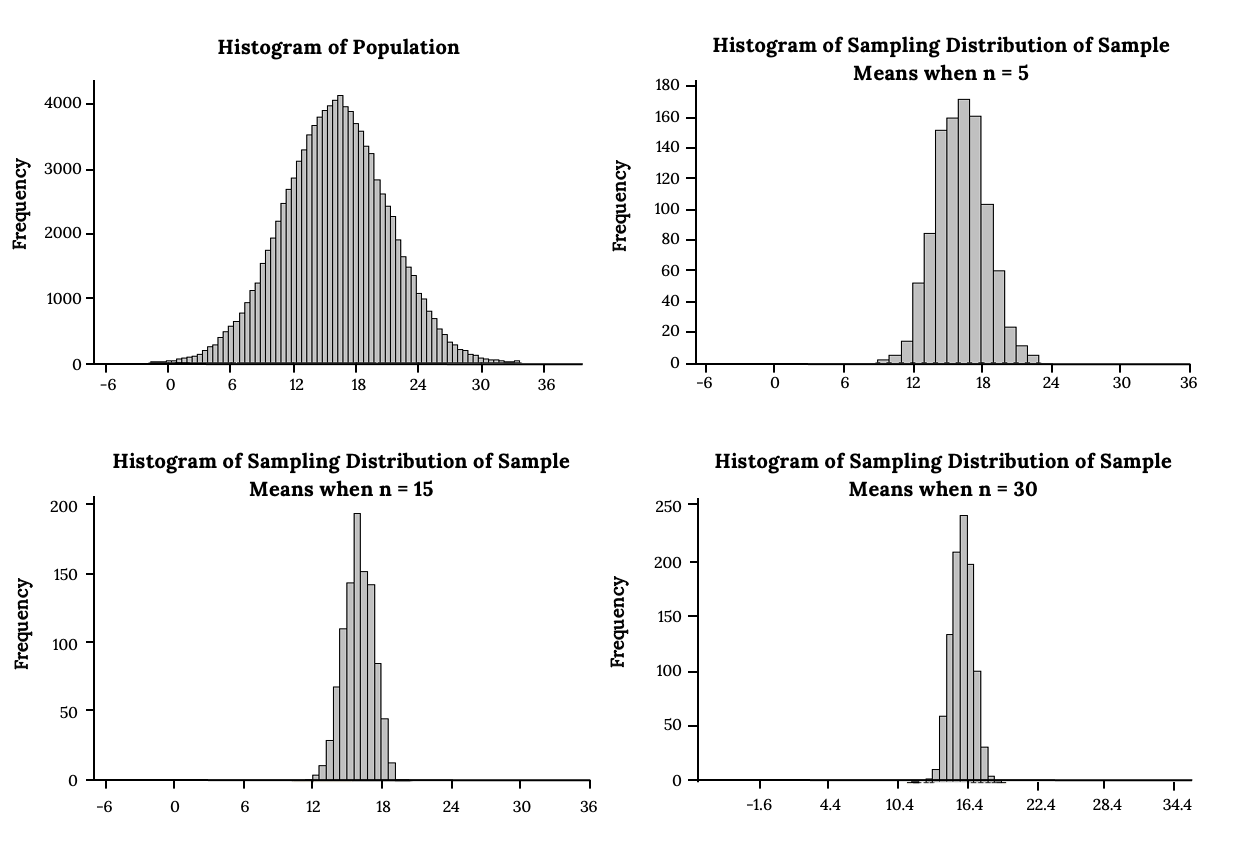
The following images look at sampling distributions of the sample mean built from taking 1000 samples of different sample sizes from a normal Population. What pattern do you notice?

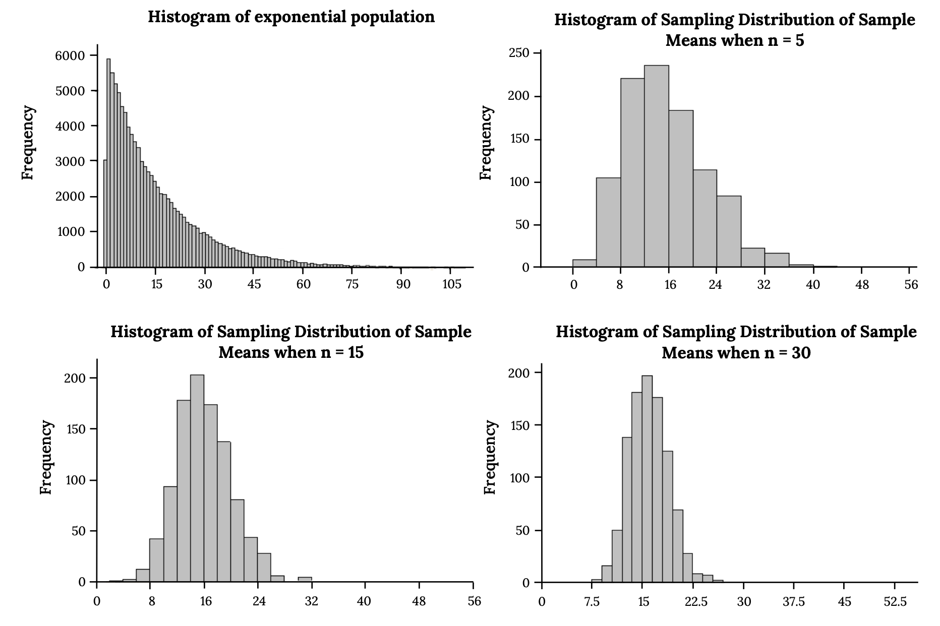
Four histograms. Top left - Histogram of Population; Top right - Histogram of Sampling Distribution of Sample Means when n = 5; Bottom left - Histogram of Sampling Distribution of Sample Means when n = 15; Bottom right - Histogram of Sampling Distribution of Sample Means when n = 30. All histograms follow typical bell-curve shape and as n increases, the shape gets more narrow around the mean. — Figure 6.4: Sampling Distributions of the Sample Mean from a Normal Population

The following images look at sampling distributions of the sample mean built from taking 1000 samples of different sample sizes from a non-normal Population (in this case it happens to be exponential). What pattern do you notice?

Four histograms. Top left - Histogram of exponential population; Top right - Histogram of Sampling Distribution of Sample Means when n = 5; Bottom left - Histogram of Sampling Distribution of Sample Means when n = 15; Bottom right - Histogram of Sampling Distribution of Sample Means when n = 30. All histograms are skewed right and as n increases, the plot gets more narrow around the mean. — Figure 6.5: Sampling Distributions of the Sample Mean from a Non-Normal Population

What differences do you notice when sampling from a normal population vs. Non normal?

Example

Suppose:

eight students roll one fair die ten times
seven roll two fair dice ten times
nine roll five fair dice ten times
11 roll ten fair dice ten times.

Each time a person rolls more than one die, he or she calculates the sample mean of the faces showing. For example, one person might roll five fair dice and get 2, 2, 3, 4, 6 on one roll.

The mean is $\frac{\text{2 + 2 + 3 + 4 + 6}}{5}$ = 3.4. The 3.4 is one mean when five fair dice are rolled. This same person would roll the five dice nine more times and calculate nine more means for a total of ten means.

As the number of dice rolled increases from one to two to five to ten, the following would happen:

The mean of the sample means remains approximately the same.
The spread of the sample means (the standard deviation of the sample means) gets smaller.
The graph appears steeper and thinner.

We have just demonstrated the idea of central limit theorem (clt) for means, that as you increase the sample size, the sampling distribution of the sample mean tends toward a normal distribution.

To summarize, the central limit theorem for sample means says that if you keep drawing larger and larger samples (such as rolling one, two, five, and finally, ten dice) and calculating their means, the sample means form their own normal distribution (the sampling distribution). The normal distribution has the same mean as the original distribution and a variance that equals the original variance divided by the sample size. Standard deviation is the square root of variance, so the standard deviation of the sampling distribution (aka standard error) is the standard deviation of the original distribution divided by the square root of n. The variable n is the number of values that are averaged together, not the number of times the experiment is done.

It would be difficult to overstate the importance of the central limit theorem in statistical theory. Knowing that data, even if its distribution is not normal, behaves in a predictable way is a powerful tool. We can simulate this idea using technology.

Suppose X is a random variable with a distribution that may be known or unknown (it can be any distribution). Using a subscript that matches the random variable, let:

μ_X = the mean of X
σ_X = the standard error of X

$\sigma_{\overline{x}}\text{ = }\frac{\sigma}{\sqrt{n}}$ = standard deviation of $\overline{x}$ and is called the standard error of the mean. Note here we are assuming we know the population standard deviation.

If you draw random samples of size n, then as n increases, the random variable $\overline{X}$ which consists of sample means, tends to be normally distributed and

$\overline{x}$ ~ N $\left({\mu }_{x}\text{, }\frac{\sigma}{\sqrt{n}}\right)$ .

To put it more formally, if you draw random samples of size n, the distribution of the random variable $\overline{X}$ , which consists of sample means, is called the sampling distribution of the sample mean. The sampling distribution of the mean approaches a normal distribution as n, the sample size, increases.

Using the CLT

It is important to understand when to use the central limit theorem:

If you are being asked to find the probability of an individual value, do not use the CLT. Use the distribution of its random variable.
If you are being asked to find the probability of the mean of a sample, then use the CLT for the mean.

The random variable $\overline{X}$ has a different z-score formula associated with it from that of a single observation. Remeber, The mean $\overline{x}$ is the mean of one sample and μ_X is the average, or center, of both X (The original distribution) and $\overline{X}$ .

$z=\frac{\overline{x}-{\mu }_{x}}{\left(\frac{{\sigma }_{x}}{\sqrt{n}}\right)}$

We can use our Z table and standardize just as we are already familiar with, or can use your technology of choice

Example

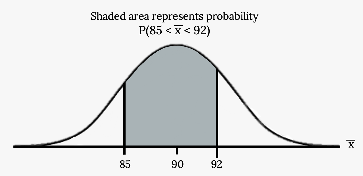
An unknown distribution has a mean of 90 and a standard deviation of 15. Samples of size n = 25 are drawn randomly from the population.

a. Find the probability that the sample mean is between 85 and 92.

Let X = one value from the original unknown population. The probability question asks you to find a probability for the sample mean.

Find P(85 < $\overline{x}$ < 92). Draw a graph.

Normal distribution curve where the peak of the curve coincides with the point 90 on the horizontal axis. The points 85 and 92 are labeled on the axis. Vertical lines are drawn from these points to the curve and the area between the lines is shaded. The shaded region represents the probability that 85 < x < 92. — Figure 6.6: Area Under the Curve

b. Find the value that is two standard deviations above the expected value, 90, of the sample mean.

Your turn!

An unknown distribution has a mean of 45 and a standard deviation of eight. Samples of size n = 30 are drawn randomly from the population. Find the probability that the sample mean is between 42 and 50.

Image References

Figure 6.4: Kindred Grey via Virginia Tech (2021). “Sampling Distributions of the Sample Mean from a Normal Population.” CC BY-SA 4.0. Retrieved from https://commons.wikimedia.org/wiki/File:Sampling_Distributions_of_the_Sample_Mean_from_a_Normal_Population.png

Figure 6.5: Kindred Grey via Virginia Tech (2021). “Sampling Distributions of the Sample Mean from a Non-Normal Population.” CC BY-SA 4.0. Retrieved from https://commons.wikimedia.org/wiki/File:Sampling_Distributions_of_the_Sample_Mean_from_a_Non-Normal_Population.png

Figure 6.6: Kindred Grey via Virginia Tech (2020). “Figure 6.4” CC BY-SA 4.0. Retrieved from https://commons.wikimedia.org/wiki/File:Figure_6.4.png . Adaptation of Figure 5.39 from OpenStax Introductory Statistics (2013) (CC BY 4.0). Retrieved from https://openstax.org/books/statistics/pages/5-practice

License

Icon for the Creative Commons Attribution-ShareAlike 4.0 International License

Significant Statistics Copyright © 2020 by John Morgan Russell, OpenStaxCollege, OpenIntro is licensed under a Creative Commons Attribution-ShareAlike 4.0 International License, except where otherwise noted.

The Central Limit Theorem for a Sample Mean

Using the CLT

License

Share This Book