6.3 Introduction to Confidence Intervals

Adapted by John Morgan Russell; from Barbara Illowsky and Susan Dean, David Diez, Mine Cetinkaya-Rundel and Christopher D. Barr; Julie Vu and David Harrington

6.3 Introduction to Confidence Intervals

White bowl with lots of M&Ms sits on a white table. — Figure 6.7: M&Ms. Have you ever wondered what the average number of M&Ms in a bag at the grocery store is? You can use confidence intervals to answer this question.

We use inferential statistics to make generalizations about an unknown population. The simplest way of doing this is to use the sample data help us to make a point estimate of a population parameter. We realize that due to sampling variability the point estimate is most likely not the exact value of the population parameter, but should be close to it. After calculating point estimates, we can build off of them to construct interval estimates, called confidence intervals.

Confidence Intervals

A confidence interval is another type of estimate but, instead of being just one number, it is an interval of numbers. It provides a range of reasonable values in which we expect the population parameter to fall. Essentially the idea is that since a point estimate may not be perfect due to variability, we will build an interval based on a point estimate to hopefully capture the parameter of interest in the interval. There is no guarantee that a given confidence interval does capture the parameter, but there is a predictable probability of success. It is important to keep in mind that the confidence interval itself is a random variable, while the population parameter is fixed.

If you worked in the marketing department of an entertainment company, you might be interested in the mean number of songs a consumer downloads a month from iTunes. If so, you could conduct a survey and calculate the sample mean, $\overline{x}$ . You would use $\overline{x}$ to estimate the population mean. The sample mean, $\overline{x}$ , is the point estimate for the population mean, μ.

Suppose, for the iTunes example, we do not know the population mean μ, but we do know that the population standard deviation is σ = 1 and our sample size is 100. Then, by the central limit theorem, the standard deviation for the sample mean is

$\frac{\sigma }{\sqrt{n}}$ = $\frac{1}{\sqrt{100}}=0.1$ .

The Empirical Rule, which applies to bell-shaped distributions, says that in approximately 95% of the samples, the sample mean, $\overline{x}$ , will be within two standard deviations of the population mean μ. For our iTunes example, two standard deviations is (2)(0.1) = 0.2. The sample mean $\overline{x}$ is likely to be within 0.2 units of μ.

Because $\overline{x}$ is within 0.2 units of μ, which is unknown, then μ is likely to be within 0.2 units of $\overline{x}$ in 95% of the samples. The population mean μ is contained in an interval whose lower number is calculated by taking the sample mean and subtracting two standard deviations (2)(0.1) and whose upper number is calculated by taking the sample mean and adding two standard deviations. In other words, μ is between $\overline{x}\text{ }-\text{ 0}\text{.2}$ and $\overline{x}\text{ }+\text{ 0}\text{.2}$ in 95% of all the samples.

For the iTunes example, suppose that a sample produced a sample mean $\overline{x}\text{ }=\text{ 2}$ . Then the unknown population mean μ is between

$\overline{x}-0.2=2-0.2=1.8$ and $\overline{x}+0.2=2+0.2=2.2$

We can say that we are about 95% confident that the unknown population mean number of songs downloaded from iTunes per month is between 1.8 and 2.2. The approximate 95% confidence interval is (1.8, 2.2).

This approximate 95% confidence interval implies two possibilities. Either the interval (1.8, 2.2) contains the true mean μ or our sample produced an $\overline{x}$ that is not within 0.2 units of the true mean μ. The second possibility happens for only 5% of all the samples (95–100%).

Remember that a confidence intervals are created for an unknown population parameter. Confidence intervals for most parameters have the form:

(Point Estimate ± Margin of Error) = (Point Estimate – Margin of Error, Point Estimate + Margin of Error)

The margin of error (MoE) depends on the confidence level or percentage of confidence and the standard error of the mean.

When you read newspapers and journals, some reports will use the phrase “margin of error.” Other reports will not use that phrase, but include a confidence interval as the point estimate plus or minus the margin of error. These are two ways of expressing the same concept.

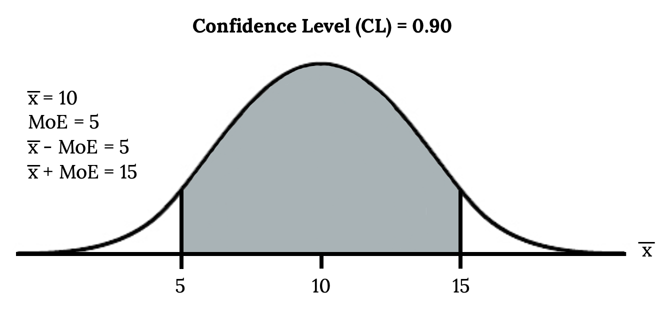
A confidence interval for a population mean with a known standard deviation is based on the fact that the sample means follow an approximately normal distribution. Suppose that our sample has a mean of $\overline{x}\text{ = 10}$ and we have constructed the 90% confidence interval (5, 15) where MoE = 5.

Calculating the Confidence Interval

To construct a confidence interval for a single unknown population mean μ, where the population standard deviation is known, we need $\overline{x}$ as an estimate for μ and we need the margin of error. Here, the margin of error (MoE). The sample mean $\overline{x}$ is the point estimate of the unknown population mean μ.

Since a confidence interval estimate will have the form:

$(PE-MoE, PE+MoE)$

Then a confidence Interval for the unknown population mean μ in symbols would look like:

$(\overline{x}-MoE,\overline{x}+MoE)$

Remember, the margin of error (MoE) depends mainly on the confidence level (abbreviated CL). The confidence level is often considered the probability that the calculated confidence interval estimate will contain the true population parameter. However, it is more accurate to state that the confidence level is the percent of confidence intervals that contain the true population parameter when repeated samples are taken. Most often, it is the choice of the person constructing the confidence interval to choose a confidence level of 90% or higher because that person wants to be reasonably certain of his or her conclusions.

There is another probability called alpha (α). α is related to the confidence level, CL and represents the chance that the interval does not contain the unknown population parameter.
Mathematically, α + CL = 1.

To construct a confidence interval estimate for an unknown population mean, we need data from a random sample. The steps to construct and interpret the confidence interval are:

Calculate the sample mean $\overline{x}$ from the sample data. Remember, in this section we already know the population standard deviation σ.
Find the z-score (Critical Value) that corresponds to the confidence level.
Calculate the margin of error (MoE).
Construct the confidence interval.
Write a sentence that interprets the estimate in the context of the situation in the problem. (Explain what the confidence interval means, in the words of the problem.)

We will first examine each step in more detail, and then illustrate the process with some examples.

Example

Suppose we have collected data from a sample. We know the sample mean but we do not know the mean for the entire population. The sample mean is seven, and the error bound for the mean is 2.5. Find the confidence interval and interpret.

Your turn!

Suppose we have data from a sample. The sample mean is 15, and the margin of error for the mean is 3.2. What is the confidence interval estimate for the population mean?

Changing the Confidence Level

A confidence interval for a population mean with a known standard deviation is based on the fact that the sample means follow an approximately normal distribution. Suppose that our sample has a mean of $\overline{x}$ = 10, and we have constructed the 90% confidence interval (5, 15) where MoE = 5.

To get a 90% confidence interval, we must include the central 90% of the probability of the normal distribution. If we include the central 90%, we leave out a total of α = 10% in both tails, or 5% in each tail, of the normal distribution.

This is a normal distribution curve. The peak of the curve coincides with the point 10 on the horizontal axis. The points 5 and 15 are labeled on the axis. Vertical lines are drawn from these points to the curve, and the region between the lines is shaded. The shaded region has area equal to 0.90. — Figure 6.8: 90% Confidence Level

To capture the central 90%, we must go out 1.645 “standard deviations” on either side of the calculated sample mean. The value 1.645 is the z-score from a standard normal probability distribution that puts an area of 0.90 in the center, an area of 0.05 in the far left tail, and an area of 0.05 in the far right tail.

It is important that the “standard deviation” used must be appropriate for the parameter we are estimating, so in this section we need to use the standard deviation that applies to sample means, which is $\frac{\sigma }{\sqrt{n}}$ . The fraction $\frac{\sigma }{\sqrt{n}}$ , is commonly called the “standard error of the mean” in order to distinguish clearly the standard deviation for a mean from the population standard deviation σ.

In summary, as a result of the central limit theorem:

$\overline{X}$ is normally distributed, that is, $\overline{X}$ ~ N $\left({\mu }_{X},\frac{\sigma }{\sqrt{n}}\right)$ .
When the population standard deviation σ is known, we use a normal distribution to calculate the margin of error.

Finding the Critical Value

When we know the population standard deviation σ, we use a standard normal distribution to calculate the margin of error (MoE) and construct the confidence interval. We need to find the value of z that puts an area equal to the confidence level (in decimal form) in the middle of the standard normal distribution Z ~ N(0, 1). This Z score is also called a critical value.

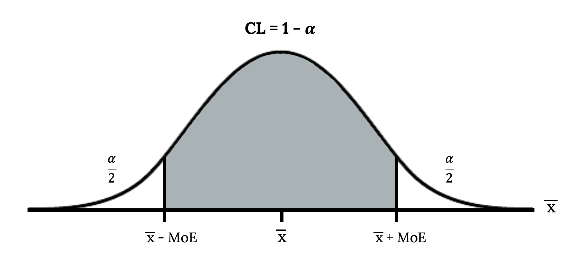
The confidence level, CL, is the area in the middle of the standard normal distribution. CL = 1 – α, so α is the area that is split equally between the two tails. Each of the tails contains an area equal to $\frac{\alpha }{2}$ .

The z-score that has an area to the right of $\frac{\alpha }{2}$ is denoted by ${z}_{\frac{\alpha }{2}}$ .

Note: Remember to use the area to the LEFT of ${z}_{\frac{\alpha }{2}}$

Example

Find the critical value for a 95% Confidence Interval:

Examples

Find the critical value for a 90% Confidence Interval

Calculating the Margin of Error (MoE)

The error bound formula for an unknown population mean μ when the population standard deviation σ is known is

MoE = $\left({z}_{\frac{\alpha }{2}}\right)\left(\frac{\sigma }{\sqrt{n}}\right)$

Constructing the Confidence Interval

A confidence interval estimate has the format:

$\left(\overline{x}-MoE,\overline{x}+MoE\right)$ .

The graph gives a picture of the entire situation.

CL + $\frac{\alpha }{2}$ + $\frac{\alpha }{2}$ = CL + α = 1.

This is a normal distribution curve. The peak of the curve coincides with the point x-bar on the horizontal axis. The points x-bar - MoE and x-bar + MoE are labeled on the axis. Vertical lines are drawn from these points to the curve, and the region between the lines is shaded. The shaded region has area equal to 1 - a and represents the confidence level. Each unshaded tail has area a/2. — Figure 6.9: Constructing the Confidence Interval

Writing the Interpretation

The interpretation should clearly state the confidence level (CL), explain what population parameter is being estimated (here the population mean), and state the confidence interval (both endpoints). “We can be % confident that the interval we created, to___ captures the true population mean (include the context of the problem and appropriate units).”

Be careful that you do not associate the confidence level with the parameter itself. Your parameter is a fixed value, what is changing is the sample you take and the interval you calculate. We always want to associate the CL% with the sampling process and the interval.

Example

Suppose scores on exams in statistics are normally distributed with an unknown population mean and a population standard deviation of three points. A random sample of 36 scores is taken and gives a sample mean (sample mean score) of 68. Find a confidence interval estimate for the population mean exam score (the mean score on all exams).

Find a 90% confidence interval for the true (population) mean of statistics exam scores.

The step-by-step solution is shown below. If you are comfortable using software, you can use it to calculate the confidence interval directly.

Your turn!

Suppose average pizza delivery times are normally distributed with an unknown population mean and a population standard deviation of six minutes. A random sample of 28 pizza delivery restaurants is taken and has a sample mean delivery time of 36 minutes.

Find a 90% confidence interval estimate for the population mean delivery time and interpret.

Image Credits

Figure 6.7: Sebastian Gomez (2020). “Yellow green and red candies” Public domain. Retrieved from https://unsplash.com/photos/w9pT3v9z1CM

Figure 6.8: Kindred Grey via Virginia Tech (2020). “Figure 6.6” CC BY-SA 4.0. Retrieved from https://commons.wikimedia.org/wiki/File:Figure_6.6.png . Adaptation of Figure 5.39 from OpenStax Introductory Statistics (2013) (CC BY 4.0). Retrieved from https://openstax.org/books/statistics/pages/5-practice

Figure 6.9: Kindred Grey via Virginia Tech (2020). “Figure 6.7” CC BY-SA 4.0. Retrieved from https://commons.wikimedia.org/wiki/File:Figure_6.7.png . Adaptation of Figure 5.39 from OpenStax Introductory Statistics (2013) (CC BY 4.0). Retrieved from https://openstax.org/books/statistics/pages/5-practice

License

Icon for the Creative Commons Attribution-ShareAlike 4.0 International License

Significant Statistics Copyright © 2020 by John Morgan Russell, OpenStaxCollege, OpenIntro is licensed under a Creative Commons Attribution-ShareAlike 4.0 International License, except where otherwise noted.

Confidence Intervals

Calculating the Confidence Interval

Changing the Confidence Level

Finding the Critical Value

Calculating the Margin of Error (MoE)

Constructing the Confidence Interval

Writing the Interpretation

Image Credits

License

Share This Book