6.1 Point Estimation and Sampling Distributions
Learning Objectives
By the end of this chapter, the student should be able to:
- Understand point estimation
- Apply and interpret the Central Limit Theorem
- Construct and interpret confidence intervals for means when the population standard deviation is known
- Understand the behavior of confidence intervals
- Carry out hypothesis tests for means when the population standard deviation is known
- Understand the probabilities of error in hypothesis tests

Statistical Inference
Statistical inference uses what we know about probability to make our best “guesses” or estimates from samples about the population they came from. The main forms of Inference are:
Point Estimation
Suppose you were trying to determine the mean rent of a two-bedroom apartment in your town. You might look in the classified section of the newspaper, write down several rents listed, and average them together. You would have obtained a point estimate of the true mean. If you are trying to determine the percentage of times you make a basket when shooting a basketball, you might count the number of shots you make and divide that by the number of shots you attempted. In this case, you would have obtained a point estimate for the true proportion.
The most natural way to estimate features of the population (parameters) is to use the corresponding summary statistic calculated from the sample. Some common point estimates and their corresponding parameters are found i n the following table:
| Parameter | Measure | Statistic |
| μ | Mean of a single population | x̅ |
| p | Proportion of a single population | ˆp |
| μD | Mean difference of two dependent populations (MP) | x̅ D |
| μ1-μ2 | Difference in means of two independent populations | x̅ 1-x̅ 2 |
| p1–p2 | Difference in proportions of two populations | ˆp1-ˆp2 |
| σ2 | Variance of a single population | S2 |
| σ | Standard deviation of a single population | S |
Suppose the mean weight of a sample of 60 adults is 173.3 lbs; this sample mean is a point estimate of the population mean weight, µ. Remember this is one of many samples that we could have taken from the population. If a different random sample of 60 individuals were taken from the same population, the new sample mean would likely be different as a result of sampling variability. While estimates generally vary from one sample to another, the population mean is a fixed value.
Suppose a poll suggested the US President’s approval rating is 45%. We would consider 45% to be a point estimate of the approval rating we might see if we collected responses from the entire population. This entire-population response proportion is generally referred to as the parameter of interest. When the parameter is a proportion, it is often denoted by p, and we often refer to the sample proportion as ˆp (pronounced “p-hat”). Unless we collect responses from every individual in the population, p remains unknown, and we use ˆp as our estimate of p.
How would one estimate the difference in average weight between men and women? Suppose a sample of men yields a mean of 185.1 lbs and a sample of women men yields a mean of 162.3 lbs. What is a good point estimate for the difference in these two population means? We will expand on this in following chapters.
Sampling Distributions
We have established that different samples yield different statistics due to sampling variability . These statistics have their own distributions, called sampling distributions, that reflect this as a random variable. The sampling distribution of a sample statistic is the distribution of the point estimates based on samples of a fixed size, n, from a certain population. It is useful to think of a particular point estimate as being drawn from a sampling distribution.
Recall the sample mean weight calculated from a previous sample of 173.3 lbs. Suppose another random sample of 60 participants might produce a different value of x, such as 169.5 lbs. Repeated random sampling could result in additional different values, perhaps 172.1 lbs, 168.5 lbs, and so on. Each sample mean can be thought of as a single observation from a random variable X. The distribution of X is called the sampling distribution of the sample mean, and has its own mean and standard deviation like the random variables discussed previously. We will simulate the concept of a sampling distribution using technology to repeatedly sample, calculate statistics, and graph them. However, the actual sampling distribution would only be attainable if we could theoretically take an infinite amount of samples.
Each of the point estimates in the table above have their own unique sampling distributions which we will look at in the future
Unbiased Estimation
Although variability in samples is present, there remains a fixed value for any population parameter. What makes a statistical estimate of this parameter of interest a “Good” one? It must be both accurate and precise.
The accuracy of an estimate refers to how well it estimates the actual value of that parameter. Mathematically, this is true when that the expected value your statistic is equal to the value of that parameter. This can be visualized as the center of the sampling distribution appearing to be situated at the value of that parameter.
According to the law of large numbers, probabilities converge to what we expect over time. Point estimates follow this rule, becoming more accurate with increasing sample size. The figure below shows the sample mean weight calculated for random samples drawn, where sample size increases by 1 for each draw until sample size equals 500. The maroon dashed horizontal line is drawn at the average weight of all adults 169.7 lbs, which represents the population mean weight according to the CDC.
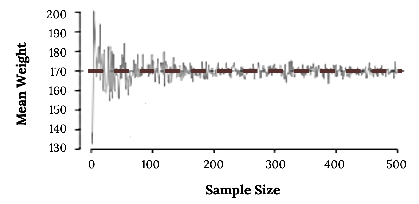
Note how a sample size around 50 may produce a sample mean that is as much as 10 lbs higher or lower than the population mean. As sample size increases, the fluctuations around the population mean decrease; in other words, as sample size increases, the sample mean becomes less variable and provides a more reliable estimate of the population mean.
In addition to accuracy, a precise estimate is also more useful. This means when repeatedly sampling, the values of the statistics seem pretty close together. The precision of an estimate can be visualized as the spread of the sampling distribution, usually quantified by the standard deviation. The phrase “the standard deviation of a sampling distribution” is often shortened to the standard error. A smaller standard error means a more precise estimate and is also effected by sample size.
Image Credits
Figure 6.1: Michael Longmire (2019). “Coins spilling out of a jar.” Public domain. Retrieved from https://unsplash.com/photos/lhltMGdohc8
Figure 6.3: Kindred Grey (2020). “Figure 6.3.” CC BY-SA 4.0. Retrieved from https://commons.wikimedia.org/wiki/File:Figure_6.3.png
Using information from a sample to answer a question, or generalize, about a population
A subset of the population studied
The whole group of individuals who can be studied to answer a research question
Using sample data to calculate a single statistic as an estimate of an unknown population parameter
An interval built around a point estimate for an unknown population parameter
A decision making procedure for determining whether sample evidence supports a hypothesis
A number that is used to represent a population characteristic and can only be calculated as the result of a census
A number calculated from a sample
The idea that samples from the same population can yield different results
The probability distribution of a statistic at a given sample size
As the number of trials in a probability experiment increases, the relative frequency of an event approaches the theoretical probability
The standard deviation of a sampling distribution
