6.5 Introduction to Hypothesis Tests

One job of a statistician is to make statistical inferences about populations based on samples taken from the population. Confidence intervals are one way to estimate a population parameter.
Another way to make a statistical inference is to make a decision about a parameter. For instance, a car dealer advertises that its new small truck gets 35 miles per gallon, on average. A tutoring service claims that its method of tutoring helps 90% of its students get an A or a B. A company says that women managers in their company earn an average of $60,000 per year. A statistician may want to make a decision about or evaluate these claims. A hypothesis test can be used to do this.
A hypothesis test involves collecting data from a sample and evaluating the data. Then, the statistician makes a decision as to whether or not there is sufficient evidence, based upon analyses of the data, to reject the null hypothesis.
In this section you will conduct hypothesis tests on single means when the population standard deviation is known.
Hypothesis testing consists of two contradictory hypotheses or statements, a decision based on the data, and a conclusion. To perform a hypothesis test, a statistician will perform some variation of these steps:
- Define hypotheses.
- Collect and/OR use the sample data to determine the correct distribution to use.
- Calculate Test Statistic.
- Make a decision
- Write a conclusion.
Defining your hypotheses
The actual test begins by considering two hypotheses. They are called the null hypothesis and the alternative hypothesis. These hypotheses contain opposing viewpoints.
The null hypothesis (H0): It is often a statement of the accepted historical value or norm. This is your starting point that you must assume from the beginning in order to show an effect exists.
The alternative hypothesis (Ha): It is a claim about the population that is contradictory to H0 and what we conclude when we reject H0.
Since the null and alternative hypotheses are contradictory, you must examine evidence to decide if you have enough evidence to reject the null hypothesis or not. The evidence is in the form of sample data.
After you have determined which hypothesis the sample supports, you make a decision. There are two options for a decision. They are “reject H0” if the sample information favors the alternative hypothesis or “do not reject H0” or “decline to reject H0” if the sample information is insufficient to reject the null hypothesis.
Mathematical symbols used in H0 and Ha:
| H0 | Ha |
|---|---|
| equal (=) | not equal (≠) or greater than (>) or less than (<) |
| greater than or equal to (≥) | less than (<) |
| less than or equal to (≤) | more than (>) |
Example
We want to test whether the mean GPA of students in American colleges is different from 2.0 (out of 4.0). The null hypothesis is: H0: μ = 2.0. What is the alternative hypothesis?
Your turn!
A medical trial is conducted to test whether or not a new medicine reduces cholesterol by 25%. State the null and alternative hypotheses.
Using the Sample to Test the Null Hypothesis
Once you have defined your hypotheses the next step in the process, is to collect sample data. In a classroom context most of the time the data or summary statistics will be given to you.
Then you will have to determine the correct distribution to perform the hypothesis test, given the assumptions you are able to make about the situation. Right now we are demonstrating these ideas in a test for a mean when the population standard deviation is known using the Z distribution. We will see other scenarios in the future.
Calculating a Test Statistic
Next, you will start evaluating the data. This begins with calculating your test statistic, which is a measure of how far what you observed is from what you are assuming to he true. In this context, your test statistic, zο, quantifies the number of standard deviations between the sample mean x and the population mean µ. Calculating the test statistic is analogous to standardizing observations with Z-scores as discussed previously:

where µo is the value assumed to be true in the null hypothesis.
Making a Decision
Once you have your test statistic there are two methods to use it to make your decision:
- Critical value method – This is one way you can make a decision, but will not be discussed in detail at this time.
- P-Value method – This is the preferred method we will focus on.
P-Value Method
To find a p-value we use the test statistic to calculate the actual probability of getting the test result. Formally, the p-value is the probability that, if the null hypothesis is true, the results from another randomly selected sample will be as extreme or more extreme as the results obtained from the given sample.
A large p-value calculated from the data indicates that we should not reject the null hypothesis. The smaller the p-value, the more unlikely the outcome, and the stronger the evidence is against the null hypothesis. We would reject the null hypothesis if the evidence is strongly against it.
Draw a graph that shows the p-value. The hypothesis test is easier to perform if you use a graph because you see the problem more clearly.
Example
Suppose a baker claims that his bread height is more than 15 cm, on average. Several of his customers do not believe him. To persuade his customers that he is right, the baker decides to do a hypothesis test. He bakes 10 loaves of bread. The mean height of the sample loaves is 17 cm. The baker knows from baking hundreds of loaves of bread that the standard deviation for the height is 0.5 cm. and the distribution of heights is normal.
The null hypothesis could be H0: μ ≤ 15
The alternate hypothesis is Ha: μ > 15
The words “is more than” translates as a “>” so “μ > 15″ goes into the alternate hypothesis. The null hypothesis must contradict the alternate hypothesis.
Since σ is known (σ = 0.5 cm.), the distribution for the population is known to be normal with mean μ = 15 and standard deviation  .
.
Suppose the null hypothesis is true (the mean height of the loaves is no more than 15 cm). Then is the mean height (17 cm) calculated from the sample unexpectedly large? The hypothesis test works by asking the question how unlikely the sample mean would be if the null hypothesis were true. The graph shows how far out the sample mean is on the normal curve. The p-value is the probability that, if we were to take other samples, any other sample mean would fall at least as far out as 17 cm.
The p-value, then, is the probability that a sample mean is the same or greater than 17 cm. when the population mean is, in fact, 15 cm. We can calculate this probability using the normal distribution for means.
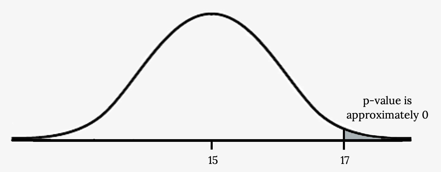
p-value= P( > 17) which is approximately zero.
A p-value of approximately zero tells us that it is highly unlikely that a loaf of bread rises no more than 15 cm, on average. That is, almost 0% of all loaves of bread would be at least as high as 17 cm. purely by CHANCE had the population mean height really been 15 cm. Because the outcome of 17 cm. is so unlikely (meaning it is happening NOT by chance alone), we conclude that the evidence is strongly against the null hypothesis (the mean height is at most 15 cm.). There is sufficient evidence that the true mean height for the population of the baker’s loaves of bread is greater than 15 cm.
Your turn!
A normal distribution has a standard deviation of 1. We want to verify a claim that the mean is greater than 12. A sample of 36 is taken with a sample mean of 12.5.
Find The P-value:
Decision and conclusion
A systematic way to make a decision of whether to reject or not reject the null hypothesis is to compare the p-value and a preset or preconceived α (also called a significance level). A preset α is the probability of a Type I error (rejecting the null hypothesis when the null hypothesis is true). It may or may not be given to you at the beginning of the problem. If there is no given preconceived α, then use α = 0.05.
When you make a decision to reject or not reject H0, do as follows:
- If α > p-value, reject H0. The results of the sample data are statistically significant. You can say there is sufficient evidence to conclude that H0 is an incorrect belief and that the alternative hypothesis, Ha, may be correct.
- If α ≤ p-value, fail to reject H0. The results of the sample data are not significant. There is not sufficient evidence to conclude that the alternative hypothesis,Ha, may be correct.
After you make your decision, write a thoughtful conclusion in the context of the scenario incorporating the hypotheses.
NOTE: When you “do not reject H0“, it does not mean that you should believe that H0 is true. It simply means that the sample data have failed to provide sufficient evidence to cast serious doubt about the truthfulness of Ho.
Example
When using the p-value to evaluate a hypothesis test, it is sometimes useful to use the following memory device
If the p-value is low, the null must go.
If the p-value is high, the null must fly.
This memory aid relates a p-value less than the established alpha (the p is low) as rejecting the null hypothesis and, likewise, relates a p-value higher than the established alpha (the p is high) as not rejecting the null hypothesis.
Fill in the blanks.
Reject the null hypothesis when .
The results of the sample data .
Do not reject the null when hypothesis when .
The results of the sample data .
Your turn!
It’s a Boy Genetics Labs claim their procedures improve the chances of a boy being born. The results for a test of a single population proportion are as follows:
H0: p = 0.50, Ha: p > 0.50
α = 0.01
p-value = 0.025
Interpret the results and state a conclusion in simple, non-technical terms.
Image Credits
Figure 6.11: Alora Griffiths (2019). “Dalmation puppy near man…” Public domain. Retrieved from https://unsplash.com/photos/7aRQZtLsvqw
Figure 6.13: Kindred Grey via Virginia Tech (2020). “Figure 6.11” CC BY-SA 4.0. Retrieved from https://commons.wikimedia.org/wiki/File:Figure_6.11.png . Adaptation of Figure 5.39 from OpenStax Introductory Statistics (2013) (CC BY 4.0). Retrieved from https://openstax.org/books/statistics/pages/5-practice
A decision making procedure for determining whether sample evidence supports a hypothesis
The claim that is assumed to be true and is tested in a hypothesis test
A working hypothesis that is contradictory to the null hypothesis
A measure of how far what you observed is from the hypothesized (or claimed) value
The probability that an event will occur, assuming the null hypothesis is true
Probability that a true null hypothesis will be rejected, also known as Type I error and denoted by α
Finding sufficient evidence that the effect we see is not just due to variability, often from rejecting the null hypothesis
