8.1 Inference for Two Dependent Samples (Matched Pairs)
Learning Objectives
By the end of this chapter, the student should be able to:
- Classify hypothesis tests by type
- Conduct and interpret hypothesis tests for two population means, population standard deviations known
- Conduct and interpret hypothesis tests for two population means, population standard deviations unknown
- Conduct and interpret hypothesis tests for matched or paired samples
- Conduct and interpret hypothesis tests for two population proportions

Studies often compare two groups. For example, maybe researchers are interested in the effect aspirin has in preventing heart attacks. One group is given aspirin and the other a placebo, and the heart attack rate is studied over several years. Other studies may compare various diet and exercise programs. Politicians compare the proportion of individuals from different income brackets who might vote for them. Students are interested in whether SAT or GRE preparatory courses really help raise their scores.
You have learned to conduct inference on single means and single proportions. We know that the first step is deciding what type of data we are working with. For quantitative data we are focused on means, while for categorical we are focused on proportions. In this chapter we will compare two means or two proportions to each other. The general procedure is still the same, just expanded. With two sample analysis it is good to know what the formulas look like and where they come from, however you will probably lean heavily on technology in preforming the calculations.
To compare two means we are obviously working with two groups, but first we need to think about the relationship between them. The groups are classified either as independent or dependent. Independent samples consist of two samples that have no relationship, that is, sample values selected from one population are not related in any way to sample values selected from the other population. Dependent samples consist of two groups that have some sort of identifiable relationship.
Two Dependent Samples (Matched Pairs)
Two samples that are dependent typically come from a matched pairs experimental design. The parameter tested using matched pairs is the population mean difference. When using inference techniques for matched or paired samples, the following characteristics should be present:
- Simple random sampling is used.
- Sample sizes are often small.
- Two measurements (samples) are drawn from the same pair of (or two extremely similar) individuals or objects.
- Differences are calculated from the matched or paired samples.
- The differences form the sample that is used for analysis.
To perform statistical inference techniques we first need to know about the sampling distribution of our parameter of interest. Remember although we start with two samples, the differences are the data we are interested in and our parameter of interest is μd, the mean difference. Our point estimate is  . In a perfect world we could assume that both samples come from a normal distribution, therefore the difference in those normal distributions are also normal. However in order to use Z, we must know the population standard deviation which is near impossible for a difference distribution. Also it is very hard to find large numbers of matched pairs so the sampling distribution we typically use for is a t distribution with n – 1 degrees of freedom, where n is the number of differences.
Confidence intervals may be calculated on their own for two samples but often, especially in the case of matched pairs, we first want to formally check to see if a difference exists with a hypothesis test. If we do find a statistically significant difference then we may estimate it with a CI after the fact.
Hypothesis Tests for the Mean difference
In a hypothesis test for matched or paired samples, subjects are matched in pairs and differences are calculated, and the population mean difference, μd, is our parameter of interest. Although it is possible to test for a certain magnitude of effect, we are most often just looking for a general effect. Our hypothesis would then look like:
Ho: μd=0
Ha: μd(<, >, ≠) 0
The steps are the same as we are familiar with, but it is tested using a Student’s-t test for a single population mean with n – 1 degrees of freedom, with the test statistic:

Example
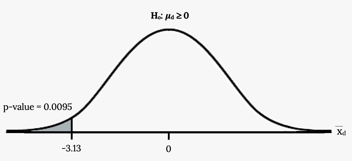
A study was conducted to investigate the effectiveness of hypnotism in reducing pain. Results for randomly selected subjects are shown in the figure below. A lower score indicates less pain. The “before” value is matched to an “after” value and the differences are calculated. The differences have a normal distribution. Are the sensory measurements, on average, lower after hypnotism? Test at a 5% significance level.
| Subject: | A | B | C | D | E | F | G | H |
|---|---|---|---|---|---|---|---|---|
| Before | 6.6 | 6.5 | 9.0 | 10.3 | 11.3 | 8.1 | 6.3 | 11.6 |
| After | 6.8 | 2.4 | 7.4 | 8.5 | 8.1 | 6.1 | 3.4 | 2.0 |
Your turn!
A study was conducted to investigate how effective a new diet was in lowering cholesterol. Results for the randomly selected subjects are shown in the table. The differences have a normal distribution. Are the subjects’ cholesterol levels lower on average after the diet? Test at the 5% level.
| Subject | A | B | C | D | E | F | G | H | I |
| Before | 209 | 210 | 205 | 198 | 216 | 217 | 238 | 240 | 222 |
| After | 199 | 207 | 189 | 209 | 217 | 202 | 211 | 223 | 201 |
Confidence Intervals for the Mean difference
The general format of a confidence interval is:

The population parameter of interest is μd, the mean difference. Our point estimate is
If we are using the t distribution, the error bound for the population mean difference is:
 ,
, is the t critical value with area to the right equal to
  ,
,- use df = n – 1 degrees of freedom, where n is the number of pairs
- sd = standard deviation of the differences.
Example
A college football coach was interested in whether the college’s strength development class increased his players’ maximum lift (in pounds) on the bench press exercise. He asked four of his players to participate in a study. The amount of weight they could each lift was recorded before they took the strength development class. After completing the class, the amount of weight they could each lift was again measured. The data are as follows:
| Weight (in pounds) | Player 1 | Player 2 | Player 3 | Player 4 |
|---|---|---|---|---|
| Amount of weight lifted prior to the class | 205 | 241 | 338 | 368 |
| Amount of weight lifted after the class | 295 | 252 | 330 | 360 |
The coach wants to know if the strength development class makes his players stronger, on average.
Using the differences data, calculate the sample mean and the sample standard deviation.
Using the difference data, this becomes a test of a single __________ (fill in the blank).
Define the random variable: mean difference in the maximum lift per player.
Graph:
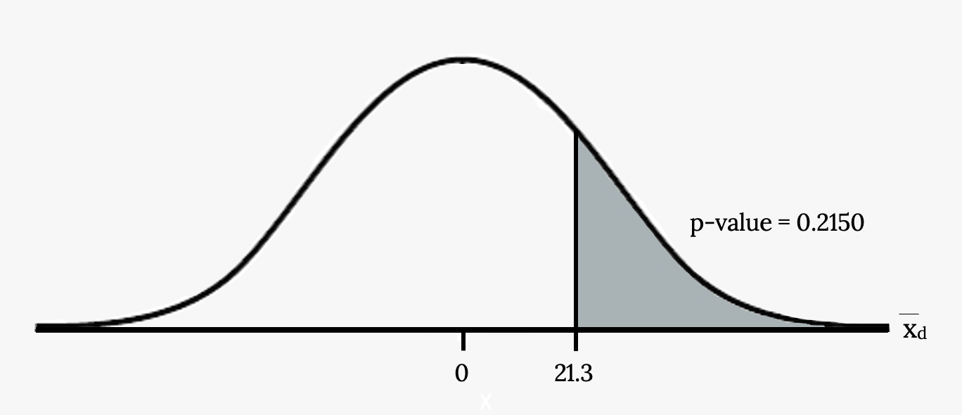
Calculate the p-value:
Decision:
What is the conclusion?
Your turn!
A new prep class was designed to improve SAT test scores. Five students were selected at random. Their scores on two practice exams were recorded, one before the class and one after. The data recorded in the figure below. Are the scores, on average, higher after the class? Test at a 5% level.
| SAT Scores | Student 1 | Student 2 | Student 3 | Student 4 |
|---|---|---|---|---|
| Score before class | 1840 | 1960 | 1920 | 2150 |
| Score after class | 1920 | 2160 | 2200 | 2100 |
Image Credits
Figure 8.1: Ali Inay (2015). “Brunching with Friends.” Public domain. Retrieved from https://unsplash.com/photos/y3aP9oo9Pjc
Figure 8.3: Kindred Grey via Virginia Tech (2020). “Figure 8.3” CC BY-SA 4.0. Retrieved from https://commons.wikimedia.org/wiki/File:Figure_8.3.png . Adaptation of Figure 5.39 from OpenStax Introductory Statistics (2013) (CC BY 4.0). Retrieved from https://openstax.org/books/statistics/pages/5-practice
Figure 8.6: Kindred Grey via Virginia Tech (2020). “Figure 8.6” CC BY-SA 4.0. Retrieved from https://commons.wikimedia.org/wiki/File:Figure_8.6.png . Adaptation of Figure 5.39 from OpenStax Introductory Statistics (2013) (CC BY 4.0). Retrieved from https://openstax.org/books/statistics/pages/5-practice
An inactive treatment that has no real effect on the explanatory variable
The facet of statistics dealing with using a sample to generalize (or infer) about the population
The arithmetic mean, or average of a population
The number of individuals that have a characteristic we are interested in divided by the total number in the population
Numerical data with a mathematical context
Data that describes qualities, or puts individuals into categories
The occurrence of one event has no effect on the probability of the occurrence of another event
Very similar individuals (or even the same individual) receive two different two treatments (or treatment vs. control) then the difference in results are compared
The mean of the differences in a matched pairs design
The probability distribution of a statistic at a given sample size
The value that is calculated from a sample used to estimate an unknown population parameter
