5.1 Introduction to Continuous Random Variables and The Uniform Distribution

Adapted by John Morgan Russell; from Barbara Illowsky and Susan Dean, David Diez, Mine Cetinkaya-Rundel and Christopher D. Barr; Julie Vu and David Harrington

5.1 Introduction to Continuous Random Variables and The Uniform Distribution

Learning Objectives

By the end of this chapter, the student should be able to:

Recognize and understand continuous probability density functions
Recognize the uniform probability distribution and apply it appropriately

Greenhouse houses many different plants that are different heights in pots. — Figure 5.1: Plant Heights. The heights of these plants are continuous random variables.

Continuous random variables have many applications. Baseball batting averages, IQ scores, the length of time a long distance telephone call lasts, the amount of money a person carries, the length of time a computer chip lasts, and SAT scores are just a few. The field of reliability depends on a variety of continuous random variables.

Note: The values of discrete and continuous random variables can be ambiguous. For example, if X is equal to the number of miles (to the nearest mile) you drive to work, then X is a discrete random variable. You count the miles. If X is the distance you drive to work, then you measure values of X and X is a continuous random variable. For a second example, if X is equal to the number of books in a backpack, then X is a discrete random variable. If X is the weight of a book, then X is a continuous random variable because weights are measured. How the random variable is defined is very important.

Properties of Continuous Probability Distributions

The graph of a continuous probability distribution is a curve. Probability is represented by area under the curve.

The curve is called the probability density function (PDF). We use the symbol f(x) to represent the curve. f(x) is the function that corresponds to the graph; we use the density function f(x) to draw the graph of the probability distribution.

Area under the curve is given by a different function called the cumulative distribution function (CDF). The cumulative distribution function is used to evaluate probability as area.

The outcomes are measured, not counted.
The entire area under the curve and above the x-axis is equal to one.
Probability is found for intervals of x values rather than for individual x values.
P(c < x < d) is the probability that the random variable X is in the interval between the values c and d. P(c < x < d) is the area under the curve, above the x-axis, to the right of c and the left of d.
P(x = c) = 0 The probability that x takes on any single individual value is zero. The area below the curve, above the x-axis, and between x = c and x = c has no width, and therefore no area (area = 0). Since the probability is equal to the area, the probability is also zero.
P(c < x < d) is the same as P(c ≤ x ≤ d) because probability is equal to area.

We will find the area that represents probability by using geometry, formulas, technology, or probability tables. In general, calculus is needed to find the area under the curve for many probability density functions however much of the work has already been done for us. The formulas to find the area in this textbook have already been found by using the techniques of integral calculus.

Some Continuous Distributions

There are many continuous probability distributions. When using a continuous probability distribution to model probability, the distribution used is selected to model and fit the particular situation in the best way. We do not often handle general CRVs, but more often study special known cases. The following graphs illustrate some of these these distributions.

Three distributions side by side. Left: Bell-shaped graph; the symmetric graph reaches maximum height at x = 0 and slopes downward gradually to the x-axis on each side of the peak. Middle: downward sloping line graph; it begins at a point on the y-axis and approaches the x-axis at the right edge of the graph. Right: The horizontal axis ranges from 0 to 10. The distribution is modeled by a rectangle extending from x = 3 to x =8. — Figure 5.2: Continuous Distributions

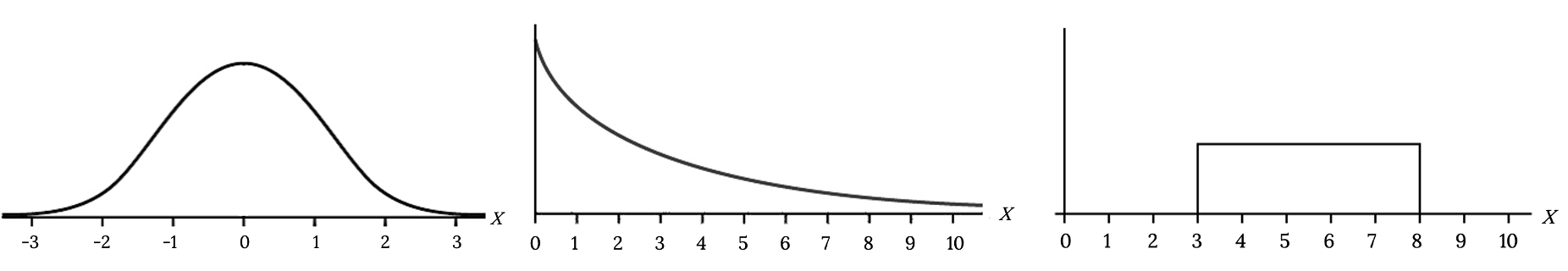
Probability Density Functions

We begin by defining a continuous probability density function. We use the function notation f(x). In the study of probability, the functions we study are special. We define the function f(x) so that the area between it and the x-axis is equal to a probability. Since the maximum probability is one, the maximum area is also one. For continuous probability distributions, you can think about it as: PROBABILITY = AREA.

The Uniform Distribution

The (continuous) uniform distribution is fairly simple and is a great place to start to demonstrate the ideas of continuous distributions. It is concerned with events that are equally likely to occur. When working out problems that have a uniform distribution, be careful to note if the data is inclusive or exclusive of endpoints.

The notation for the uniform distribution is X ~ U(a, b) where a = the lowest value of x and b = the highest value of x.

The probability density function is f(x) = $\frac{1}{b-a}$ for a ≤ x ≤ b.

Formulas for the theoretical mean and standard deviation are

$\mu =\frac{a+b}{2}$ and $\sigma =\sqrt{\frac{{\left(b-a\right)}^{2}}{12}}$

Consider the following example.

Example

The following data are 55 smiling times, in seconds, of an eight-week-old baby.

Figure 5.3: Smiling Times
10.4	19.6	18.8	13.9	17.8	16.8	21.6	17.9	12.5	11.1	4.9
12.8	14.8	22.8	20.0	15.9	16.3	13.4	17.1	14.5	19.0	22.8
1.3	0.7	8.9	11.9	10.9	7.3	5.9	3.7	17.9	19.2	9.8
5.8	6.9	2.6	5.8	21.7	11.8	3.4	2.1	4.5	6.3	10.7
8.9	9.4	9.4	7.6	10.0	3.3	6.7	7.8	11.6	13.8	18.6

The sample mean = 11.49 and the sample standard deviation = 6.23.

We will assume that the smiling times, in seconds, follow a uniform distribution between zero and 23 seconds, inclusive. This means that any smiling time from zero to and including 23 seconds is equally likely. The histogram that could be constructed from the sample is an empirical distribution that closely matches the theoretical uniform distribution.

Let X = length, in seconds, of an eight-week-old baby’s smile.

For this example, X ~ U(0, 23) and f(x) = $\frac{1}{23-0}$ for 0 ≤ X ≤ 23.

For this problem, the theoretical mean and standard deviation are

μ = $\frac{0\text{ }+\text{ }23}{2}}$ = 11.50 seconds and σ = $\sqrt{\frac{{\left(23\text{ }-\text{ }0\right)}^{2}}{12}}}$ = 6.64 seconds.

Notice that the theoretical mean and standard deviation are close to the sample mean and standard deviation in this example.

Example

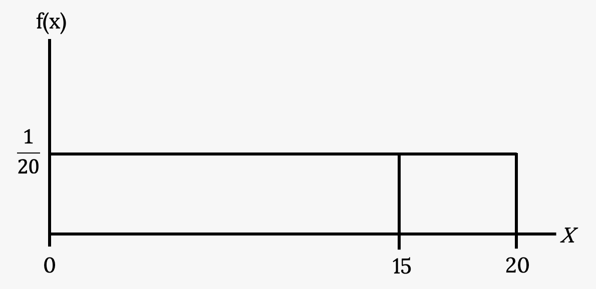
Consider the function f(x) = $\frac{1}{20}$ for 0 ≤ x ≤ 20.

x = a real number
The graph of f(x) = $\frac{1}{20}$ is a horizontal line. However, since 0 ≤ x ≤ 20, f(x) is restricted to the portion between x = 0 and x = 20, inclusive.

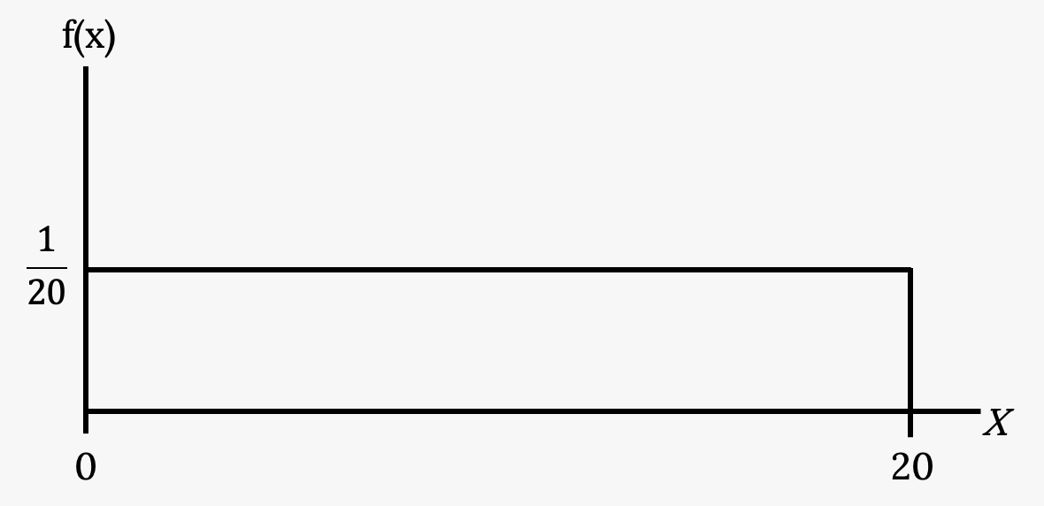
This shows the graph of the function f(x) = 1/20. A horiztonal line ranges from the point (0, 1/20) to the point (20, 1/20). A vertical line extends from the x-axis to the end of the line at point (20, 1/20) creating a rectangle. — Figure 5.4: Example of a Function

f(x) = $\frac{1}{20}$ for 0 ≤ x ≤ 20.
The graph of f(x) = $\frac{1}{20}$ is a horizontal line segment when 0 ≤ x ≤ 20.
The area between f(x) = $\frac{1}{20}$ where 0 ≤ x ≤ 20 and the x-axis is the area of a rectangle with base = 20 and height = $\frac{1}{20}$ .
$\text{AREA}=20\left(\frac{1}{20}\right)=1$

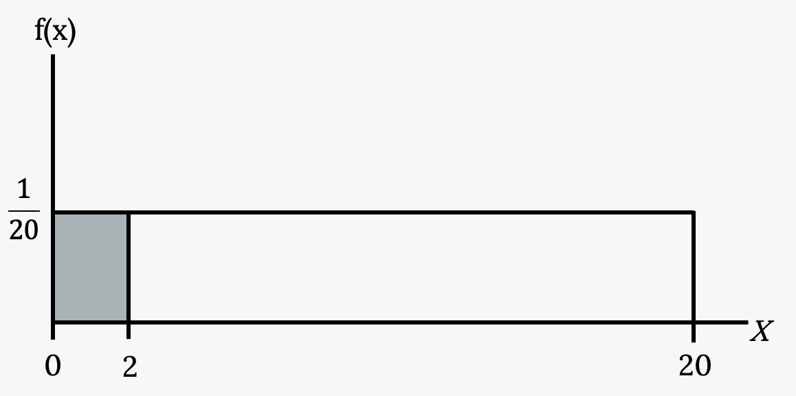
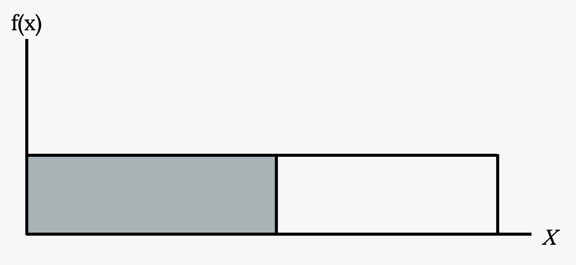
Suppose we want to find the area between f(x) = $\frac{1}{20}$ and the x-axis where 0 < x < 2.

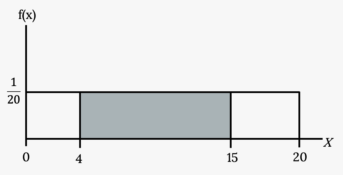
Suppose we want to find the area between f(x) = $\frac{1}{20}$ and the x-axis where 4 < x < 15.

Suppose we want to find P(x = 15).

P(X ≤ x), which can also be written as P(X < x) for continuous distributions, is called the cumulative distribution function or CDF. Notice the “less than or equal to” symbol. We can also use the CDF to calculate P(X > x). The CDF gives “area to the left” and P(X > x) gives “area to the right.” We calculate P(X > x) for continuous distributions as follows: P(X > x) = 1 – P (X < x).

Label the graph with f(x) and x. Scale the x and y axes with the maximum x and y values.

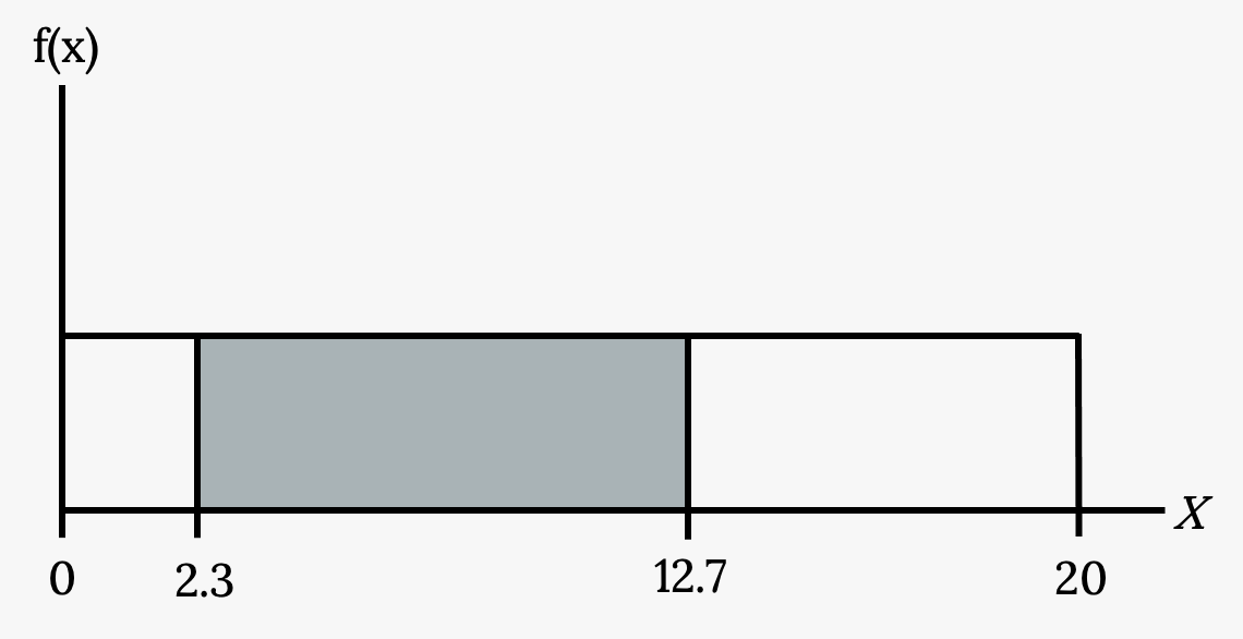
To calculate the probability that x is between two values, look at the graph above. Shade the region between x = 2.3 and x = 12.7. Then calculate the shaded area of a rectangle.

Your turn!

Consider the function f(x) = $\frac{\text{1}}{8}$ for 0 ≤ x ≤ 8. Draw the graph of f(x) and find P(2.5 < x < 7.5).

Image References

Figure 5.1: Annie Spratt (2018). “Greenhouse / glasshouse.” Public domain. Retrieved from https://unsplash.com/photos/r1yuNMUw6Lo

Figure 5.2: Kindred Grey via Virginia Tech (2020). “Figure 5.2” CC BY-SA 4.0. Retrieved from https://commons.wikimedia.org/wiki/File:Figure_5.2.png . Adaptation of Figures 5.37, 5.38, and 5.39 from OpenStax Introductory Statistics (2013) (CC BY 4.0). Retrieved from https://openstax.org/books/statistics/pages/5-practice

Figure 5.4: Kindred Grey (2020). “Figure 5.4.” CC BY-SA 4.0. Retrieved from https://commons.wikimedia.org/wiki/File:Figure_5.4.png

Figure 5.5: Kindred Grey (2020). “Figure 5.5.” CC BY-SA 4.0. Retrieved from https://commons.wikimedia.org/wiki/File:Figure_5.5.png

Figure 5.6: Kindred Grey (2020). “Figure 5.6.” CC BY-SA 4.0. Retrieved from https://commons.wikimedia.org/wiki/File:Figure_5.6.png

Figure 5.7: Kindred Grey (2020). “Figure 5.7.” CC BY-SA 4.0. Retrieved from https://commons.wikimedia.org/wiki/File:Figure_5.7.png

Figure 5.8: Kindred Grey (2020). “Figure 5.8.” CC BY-SA 4.0. Retrieved from https://commons.wikimedia.org/wiki/File:Figure_5.8.png

Figure 5.9: Kindred Grey (2020). “Figure 5.9.” CC BY-SA 4.0. Retrieved from https://commons.wikimedia.org/wiki/File:Figure_5.9.png

License

Icon for the Creative Commons Attribution-ShareAlike 4.0 International License

Significant Statistics Copyright © 2020 by John Morgan Russell, OpenStaxCollege, OpenIntro is licensed under a Creative Commons Attribution-ShareAlike 4.0 International License, except where otherwise noted.