Chapter 6 Wrap Up
Concept Check
Section Reviews
6.1 Point Estimation and Sampling Distributions
Since Populations are typically large and a census may not be feasible, we often use sample statistics to estimate population parameters. Some examples of point estimates are:
 is a point estimate for μ
- p̂ is a point estimate for ρ
- s is a point estimate for σ
However, we know sampling variability exists, so each statistic has it’s own probability distribution called a sampling distribution. In order for the statistic to be unbiased, the center of this sampling distribution should be equal to the parameter of interest (accurate), and the standard error tells us about the precision of the estimate.
6.2 Sampling Distribution of the Sample Mean
In a population whose distribution may be known or unknown, if the size (n) of samples is sufficiently large, the distribution of the sample means will be approximately normal. The mean of the sample means will equal the population mean. The standard deviation of the distribution of the sample means, called the standard error of the mean, is equal to the population standard deviation divided by the square root of the sample size (n).
The Central Limit Theorem for Sample Means:  ~ N
~ N
The Mean : μx
Central Limit Theorem for Sample Means z-score and standard error of the mean: 
Standard Error of the Mean (Standard Deviation (): 
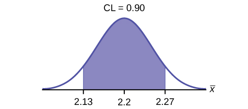
6.3 Intro to Confidence Intervals
In this module, we learned how to calculate the confidence interval for a single population mean where the population standard deviation is known. A confidence interval is made up of the point estimate with a Margin of Error built in (MoE) A CI has the general form:
(lower bound, upper bound) = (point estimate – MoE, point estimate + MoE)
The calculation of the MoE depends on the size of the sample and the level of confidence desired. The confidence level is the percent of all possible samples that can be expected to include the true population parameter. As the confidence level increases, the corresponding MoE increases as well. As the sample size increases, the MoE decreases. By the central limit theorem,

Given a confidence interval, you can work backwards to find the error bound (MoE) or the sample mean. To find the error bound, find the difference of the upper bound of the interval and the mean. If you do not know the sample mean, you can find the error bound by calculating half the difference of the upper and lower bounds. To find the sample mean given a confidence interval, find the difference of the upper bound and the error bound. If the error bound is unknown, then average the upper and lower bounds of the confidence interval to find the sample mean.
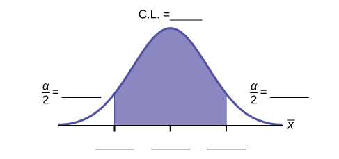
CL = confidence level, or the proportion of confidence intervals created that are expected to contain the true population parameter
α = 1 – CL = the proportion of confidence intervals that will not contain the population parameter
For a Single Population Mean with known Standard Deviation we can use the Normal Distribution. assuming the CLT holds
 = the z-score with the property that the area to the right of the z-score is
  this is the z-score used in the calculation of “MoE where α = 1 – CL.
6.4 Behavior of Confidence Intervals
If you want to increase your confidence level, the interval will increase in width all other things held constant. In order to make your interval smaller (more precise) you have to increase the sample size.
Sometimes researchers know in advance that they want to estimate a population mean within a specific margin of error for a given level of confidence. In that case, solve the MoE formula for n to discover the size of the sample that is needed to achieve this goal:

6.5 Intro to Hypothesis Tests
When the probability of an event occurring is low, and it happens, it is called a rare event. Rare events are important to consider in hypothesis testing because they can inform your willingness not to reject or to reject a null hypothesis. To test a null hypothesis, find the p-value for the sample data and graph the results. When deciding whether or not to reject the null the hypothesis, keep these two parameters in mind:
- α > p-value, reject the null hypothesis
- α ≤ p-value, do not reject the null hypothesis
In a hypothesis test, sample data is evaluated in order to arrive at a decision about some type of claim. If certain conditions about the sample are satisfied, then the claim can be evaluated for a population. In a hypothesis test, we:
- Evaluate the null hypothesis, typically denoted with H0. The null is not rejected unless the hypothesis test shows otherwise. The null statement must always contain some form of equality (=, ≤ or ≥)
- Always write the alternative hypothesis, typically denoted with Ha or H1, using less than, greater than, or not equals symbols, i.e., (≠, >, or <).
- If we reject the null hypothesis, then we can assume there is enough evidence to support the alternative hypothesis.
- Never state that a claim is proven true or false. Keep in mind the underlying fact that hypothesis testing is based on probability laws; therefore, we can talk only in terms of non-absolute certainties.
H0 and Ha are contradictory.
| If Ho has: | equal (=) | greater than or equal to (≥) | less than or equal to (≤) |
| then Ha has: | not equal (≠) or greater than (>) or less than (<) | less than (<) | greater than (>) |
If α ≤ p-value, then do not reject H0.
If α > p-value, then reject H0.
α is preconceived. Its value is set before the hypothesis test starts. The p-value is calculated from the data.
6.6 Hypothesis Tests in Depth
In every hypothesis test, the outcomes are dependent on a correct interpretation of the data. Incorrect calculations or misunderstood summary statistics can yield errors that affect the results. A Type I error occurs when a true null hypothesis is rejected. A Type II error occurs when a false null hypothesis is not rejected.
The probabilities of these errors are denoted by the Greek letters α and β, for a Type I and a Type II error respectively. The power of the test, 1 – β, quantifies the likelihood that a test will yield the correct result of a true alternative hypothesis being accepted. A high power is desirable.
α = probability of a Type I error = P(Type I error) = probability of rejecting the null hypothesis when the null hypothesis is true.
β = probability of a Type II error = P(Type II error) = probability of not rejecting the null hypothesis when the null hypothesis is false.
Key Terms
Try to define the terms below on your own. Scroll over any term to check your response!
6.1 Point Estimation and Sampling Distributions
- Statistical inference
- Sample
- Population
- Point estimation
- Hypothesis testing
- Point estimate
- Parameter
- Statistic
- Sampling variability
- Sampling distribution
- Law of large numbers
- Standard error
6.2 Sampling Distribution of the Sample Mean
6.3 Intro to Confidence Intervals
- Inferential statistics
- Population
- Point estimate
- Parameter
- Sampling variability
- Confidence interval
- Empirical rule
- Margin of error
- Critical value
6.4 Behavior of Confidence Intervals
6.5 Intro to Hypothesis Tests
- Hypothesis test
- Null hypothesis
- Alternative hypothesis
- Test statistic
- P-value
- Significance level
- Statistically significant
6.6 Hypothesis Tests in Depth
Extra Practice
6.1 Point Estimation and Sampling Distributions
1. The Specific Absorption Rate (SAR) for a cell phone measures the amount of radio frequency (RF) energy absorbed by the user’s body when using the handset. Every cell phone emits RF energy. Different phone models have different SAR measures. To receive certification from the Federal Communications Commission (FCC) for sale in the United States, the SAR level for a cell phone must be no more than 1.6 watts per kilogram. The figure below shows the highest SAR level for a random selection of cell phone models as measured by the FCC.[1] Find a point estimate of the true (population) mean of the Specific Absorption Rates (SARs) for cell phones.
| Phone Model | SAR | Phone Model | SAR | Phone Model | SAR |
|---|---|---|---|---|---|
| Apple iPhone 4S | 1.11 | LG Ally | 1.36 | Pantech Laser | 0.74 |
| BlackBerry Pearl 8120 | 1.48 | LG AX275 | 1.34 | Samsung Character | 0.5 |
| BlackBerry Tour 9630 | 1.43 | LG Cosmos | 1.18 | Samsung Epic 4G Touch | 0.4 |
| Cricket TXTM8 | 1.3 | LG CU515 | 1.3 | Samsung M240 | 0.867 |
| HP/Palm Centro | 1.09 | LG Trax CU575 | 1.26 | Samsung Messager III SCH-R750 | 0.68 |
| HTC One V | 0.455 | Motorola Q9h | 1.29 | Samsung Nexus S | 0.51 |
| HTC Touch Pro 2 | 1.41 | Motorola Razr2 V8 | 0.36 | Samsung SGH-A227 | 1.13 |
| Huawei M835 Ideos | 0.82 | Motorola Razr2 V9 | 0.52 | SGH-a107 GoPhone | 0.3 |
| Kyocera DuraPlus | 0.78 | Motorola V195s | 1.6 | Sony W350a | 1.48 |
| Kyocera K127 Marbl | 1.25 | Nokia 1680 | 1.39 | T-Mobile Concord | 1.38 |
Solution:
The sample mean is: 
2. A student polls his school to see if students in the school district are for or against the new legislation regarding school uniforms. She surveys 600 students and finds that 480 are against the new legislation. Find a point estimate of the true (population) proportion of students in the school district who are against the new legislation.
Solution:
The sample proportion is: 
6.2 Sampling Distribution of the Sample Mean
1. The length of time, in hours, it takes an “over 40” group of people to play one soccer match is normally distributed with a mean of two hours and a standard deviation of 0.5 hours. A sample of size n = 50 is drawn randomly from the population. Find the probability that the sample mean is between 1.8 hours and 2.3 hours.
- Let X = the time, in hours, it takes to play one soccer match.
- The probability question asks you to find a probability for the sample mean time, in hours, it takes to play one soccer match.
- Let = the mean time, in hours, it takes to play one soccer match.
a. If μX = _________, σX = __________, and n = ___________, then X ~ N(______, ______) by the central limit theorem for means.
- μX = 2, σX = 0.5, n = 50, and X ~ N(2,

b. Find P(1.8 < < 2.3). Draw a graph.
- P(1.8 < < 2.3) = 0.9977
normalcdf = 0.9977
- The probability that the mean time is between 1.8 hours and 2.3 hours is 0.9977.
2. The length of time taken on the SAT for a group of students is normally distributed with a mean of 2.5 hours and a standard deviation of 0.25 hours.[2] A sample size of n = 60 is drawn randomly from the population. Find the probability that the sample mean is between two hours and three hours.
3. In a recent study reported Oct. 29, 2012 on the Flurry Blog, the mean age of tablet users is 34 years.[3] Suppose the standard deviation is 15 years. Take a sample of size n = 100.
- What are the mean and standard deviation for the sample mean ages of tablet users?
- What does the distribution look like?
- Find the probability that the sample mean age is more than 30 years (the reported mean age of tablet users in this particular study).
- Find the 95th percentile for the sample mean age (to one decimal place).
Solutions:
- Since the sample mean tends to target the population mean, we have μχ = μ = 34. The sample standard deviation is given by σχ =
 =
=  =
=  = 1.5
= 1.5 - The central limit theorem states that for large sample sizes(n), the sampling distribution will be approximately normal.
- The probability that the sample mean age is more than 30 is given by P(Χ > 30) =
normalcdf(30,E99,34,1.5) = 0.9962 - Let k = the 95th percentile.
k = invNorm = 36.5
4. In an article on Flurry Blog, a gaming marketing gap for men between the ages of 30 and 40 is identified.[4] You are researching a startup game targeted at the 35-year-old demographic. Your idea is to develop a strategy game that can be played by men from their late 20s through their late 30s. Based on the article’s data, industry research shows that the average strategy player is 28 years old with a standard deviation of 4.8 years. You take a sample of 100 randomly selected gamers. If your target market is 29- to 35-year-olds, should you continue with your development strategy?
The mean number of minutes for app engagement by a tablet user is 8.2 minutes. Suppose the standard deviation is one minute. Take a sample of 60.
- What are the mean and standard deviation for the sample mean number of app engagement by a tablet user?
- What is the standard error of the mean?
- Find the 90th percentile for the sample mean time for app engagement for a tablet user. Interpret this value in a complete sentence.
- Find the probability that the sample mean is between eight minutes and 8.5 minutes.
5. Cans of a cola beverage claim to contain 16 ounces. The amounts in a sample are measured and the statistics are n = 34, = 16.01 ounces. If the cans are filled so that μ = 16.00 ounces (as labeled) and σ = 0.143 ounces, find the probability that a sample of 34 cans will have an average amount greater than 16.01 ounces. Do the results suggest that cans are filled with an amount greater than 16 ounces?
6. Yoonie is a personnel manager in a large corporation. Each month she must review 16 of the employees. From past experience, she has found that the reviews take her approximately four hours each to do with a population standard deviation of 1.2 hours. Let Χ be the random variable representing the time it takes her to complete one review. Assume Χ is normally distributed. Let be the random variable representing the mean time to complete the 16 reviews. Assume that the 16 reviews represent a random set of reviews.
a. What is the mean, standard deviation, and sample size?
- Solution: mean = 4 hours; standard deviation = 1.2 hours; sample size = 16
b. Complete the distributions.
X ~ _____(_____,_____)
~ _____(_____,_____)
- Solution: X ~ N(4, 1.2).
- Solution: X ¯ ~ N ( 4, 1.2 16 )
c. Find the probability that one review will take Yoonie from 3.5 to 4.25 hours. Sketch the graph, labeling and scaling the horizontal axis. Shade the region corresponding to the probability.
-
Figure 6.17 - P(________ < x < ________) = _______
- Solution: 3.5, 4.25, 0.2441
d. Find the probability that the mean of a month’s reviews will take Yoonie from 3.5 to 4.25 hrs. Sketch the graph, labeling and scaling the horizontal axis. Shade the region corresponding to the probability.
-
Figure 6.18 - P(________________) = _______
- Solution: 0.7499
e. What causes the probabilities in C and D to be different?
- Solution: The fact that the two distributions are different accounts for the different probabilities.
f. Find the 95th percentile for the mean time to complete one month’s reviews. Sketch the graph.
-
Figure 6.19 - The 95th Percentile =____________
- Solution: P(3.5 < x ¯ < 4.25) =
invNorm( 95,4, 1.2 16 ) = 4.49
7. Previously, De Anza statistics students estimated that the amount of change daytime statistics students carry is exponentially distributed with a mean of 88 cents. Suppose that we randomly pick 25 daytime statistics students.
- In words, Χ = ____________
- Χ ~ _____(_____,_____)
- In words, = ____________
- ~ ______ (______, ______)
- Find the probability that an individual had between $0.80 and $1.00. Graph the situation, and shade in the area to be determined.
- Find the probability that the average of the 25 students was between $0.80 and $1.00. Graph the situation, and shade in the area to be determined.
- Explain why there is a difference in part e and part f.
Solutions:
- Χ = amount of change students carry
- Χ ~ E(0.88, 0.88)
- = average amount of change carried by a sample of 25 students.
- ~ N(0.88, 0.176)
- 0.0819
- 0.1882
- The distributions are different. Part a is exponential and part b is normal.
8. Suppose that the distance of fly balls hit to the outfield (in baseball) is normally distributed with a mean of 250 feet and a standard deviation of 50 feet. We randomly sample 49 fly balls.
- If = average distance in feet for 49 fly balls, then ~ _______(_______,_______)
- What is the probability that the 49 balls traveled an average of less than 240 feet? Sketch the graph. Scale the horizontal axis for . Shade the region corresponding to the probability. Find the probability.
- Find the 80th percentile of the distribution of the average of 49 fly balls.
Solutions:
- N ( 250, 50 49 )
- 0.0808
- 256.01 feet
9. According to the Internal Revenue Service, the average length of time for an individual to complete (keep records for, learn, prepare, copy, assemble, and send) IRS Form 1040 is 10.53 hours (without any attached schedules). The distribution is unknown. Let us assume that the standard deviation is two hours. Suppose we randomly sample 36 taxpayers.
- In words, Χ = _____________
- In words, = _____________
- ~ _____(_____,_____)
- Would you be surprised if the 36 taxpayers finished their Form 1040s in an average of more than 12 hours? Explain why or why not in complete sentences.
- Would you be surprised if one taxpayer finished his or her Form 1040 in more than 12 hours? In a complete sentence, explain why.
Solutions:
- length of time for an individual to complete IRS form 1040, in hours.
- mean length of time for a sample of 36 taxpayers to complete IRS form 1040, in hours.
- N

- Yes. I would be surprised, because the probability is almost 0.
- No. I would not be totally surprised because the probability is 0.2312
10. Suppose that a category of world-class runners are known to run a marathon (26 miles) in an average of 145 minutes with a standard deviation of 14 minutes. Consider 49 of the races. Let the average of the 49 races.
- ~ _____(_____,_____)
- Find the probability that the runner will average between 142 and 146 minutes in these 49 marathons.
- Find the 80th percentile for the average of these 49 marathons.
- Find the median of the average running times.
Solutions:
- N ( 145, 14 49 )
- 0.6247
- 146.68
- 145 minutes
11. The length of songs in a collector’s iTunes album collection is uniformly distributed from two to 3.5 minutes. Suppose we randomly pick five albums from the collection. There are a total of 43 songs on the five albums.
- In words, Χ = _________
- Χ ~ _____________
- In words, = _____________
- ~ _____(_____,_____)
- Find the first quartile for the average song length, .
- The IQR (interquartile range) for the average song length, , is from ___ – ___.
Solutions:
- the length of a song, in minutes, in the collection
- U(2, 3.5)
- the average length, in minutes, of the songs from a sample of five albums from the collection
- N(2.75, 0.0660)
- 2.71 minutes
- 0.09 minutes
12. In 1940 the average size of a U.S. farm was 174 acres.[5] Let’s say that the standard deviation was 55 acres. Suppose we randomly survey 38 farmers from 1940.
- In words, Χ = _____________
- In words, = _____________
- ~ _____(_____,_____)
- The IQR for is from _______ acres to _______ acres.
Solutions:
- the size of a U.S. farm in 1940 the average size of a U.S. farm, in acres
- N ( 174, 55 38 )
- 168.0, 180.0
13. Determine which of the following are true and which are false. Then, in complete sentences, justify your answers.
- When the sample size is large, the mean of is approximately equal to the mean of Χ.
- When the sample size is large, is approximately normally distributed.
- When the sample size is large, the standard deviation of is approximately the same as the standard deviation of Χ.
Solutions:
- True. The mean of a sampling distribution of the means is approximately the mean of the data distribution.
- True. According to the Central Limit Theorem, the larger the sample, the closer the sampling distribution of the means becomes normal.
- The standard deviation of the sampling distribution of the means will decrease making it approximately the same as the standard deviation of X as the sample size increases.
14. The percent of fat calories that a person in America consumes each day is normally distributed with a mean of about 36 and a standard deviation of about ten.[6] Suppose that 16 individuals are randomly chosen. Let = average percent of fat calories.
- ~ ______(______, ______)
- For the group of 16, find the probability that the average percent of fat calories consumed is more than five. Graph the situation and shade in the area to be determined.
- Find the first quartile for the average percent of fat calories.
Solutions:
- N ( 36, 10 16 )
- 1
- 34.31
15. The distribution of income in some Third World countries is considered wedge shaped (many very poor people, very few middle income people, and even fewer wealthy people). Suppose we pick a country with a wedge shaped distribution. Let the average salary be $2,000 per year with a standard deviation of $8,000. We randomly survey 1,000 residents of that country.
- In words, Χ = _____________
- In words, = _____________
- ~ _____(_____,_____)
- How is it possible for the standard deviation to be greater than the average?
- Why is it more likely that the average of the 1,000 residents will be from $2,000 to $2,100 than from $2,100 to $2,200?
Solutions:
- X = the yearly income of someone in a third world country
- the average salary from samples of 1,000 residents of a third world country
- ∼ N

- Very wide differences in data values can have averages smaller than standard deviations.
- The distribution of the sample mean will have higher probabilities closer to the population mean.
P(2000 < < 2100) = 0.1537
P(2100 < < 2200) = 0.1317
16. Which of the following is NOT TRUE about the distribution for averages?
- The mean, median, and mode are equal.
- The area under the curve is one.
- The curve never touches the x-axis.
- The curve is skewed to the right.
Solution: d
17. The cost of unleaded gasoline in the Bay Area once followed an unknown distribution with a mean of $4.59 cents and a standard deviation of 10 cents. Sixteen gas stations from the Bay Area are randomly chosen. We are interested in the average cost of gasoline for the 16 gas stations. The distribution to use for the average cost of gasoline for the 16 gas stations is:
- ~ N(4.59, 0.10)
- ~ N(4.59,
 )
) - ~ N(4.59,
 )
) - ~ N(4.59,
 )
)
Solution: b
6.3 Intro to Confidence Intervals
1. The Specific Absorption Rate (SAR) for a cell phone measures the amount of radio frequency (RF) energy absorbed by the user’s body when using the handset. Every cell phone emits RF energy. Different phone models have different SAR measures. To receive certification from the Federal Communications Commission (FCC) for sale in the United States, the SAR level for a cell phone must be no more than 1.6 watts per kilogram. The figure below shows the highest SAR level for a random selection of cell phone models as measured by the FCC.[7] Find a 98% confidence interval for the true (population) mean of the Specific Absorption Rates (SARs) for cell phones. Assume that the population standard deviation is σ = 0.337.
| Phone Model | SAR | Phone Model | SAR | Phone Model | SAR |
|---|---|---|---|---|---|
| Apple iPhone 4S | 1.11 | LG Ally | 1.36 | Pantech Laser | 0.74 |
| BlackBerry Pearl 8120 | 1.48 | LG AX275 | 1.34 | Samsung Character | 0.5 |
| BlackBerry Tour 9630 | 1.43 | LG Cosmos | 1.18 | Samsung Epic 4G Touch | 0.4 |
| Cricket TXTM8 | 1.3 | LG CU515 | 1.3 | Samsung M240 | 0.867 |
| HP/Palm Centro | 1.09 | LG Trax CU575 | 1.26 | Samsung Messager III SCH-R750 | 0.68 |
| HTC One V | 0.455 | Motorola Q9h | 1.29 | Samsung Nexus S | 0.51 |
| HTC Touch Pro 2 | 1.41 | Motorola Razr2 V8 | 0.36 | Samsung SGH-A227 | 1.13 |
| Huawei M835 Ideos | 0.82 | Motorola Razr2 V9 | 0.52 | SGH-a107 GoPhone | 0.3 |
| Kyocera DuraPlus | 0.78 | Motorola V195s | 1.6 | Sony W350a | 1.48 |
| Kyocera K127 Marbl | 1.25 | Nokia 1680 | 1.39 | T-Mobile Concord | 1.38 |
Solution:
To find the confidence interval, start by finding the point estimate: the sample mean.
Next, find the EBM. Because you are creating a 98% confidence interval, CL = 0.98.
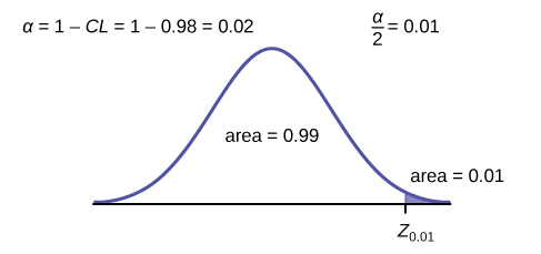
You need to find z0.01 having the property that the area under the normal density curve to the right of z0.01 is 0.01 and the area to the left is 0.99. Use your calculator, a computer, or a probability table for the standard normal distribution to find z0.01 = 2.326.

To find the 98% confidence interval, find  .
.
– EBM = 1.024 – 0.1431 = 0.8809
– EBM = 1.024 – 0.1431 = 1.1671
We estimate with 98% confidence that the true SAR mean for the population of cell phones in the United States is between 0.8809 and 1.1671 watts per kilogram.
2. The figure below shows a different random sampling of 20 cell phone models. Use this data to calculate a 93% confidence interval for the true mean SAR for cell phones certified for use in the United States.[8] As previously, assume that the population standard deviation is σ = 0.337.
| Phone Model | SAR | Phone Model | SAR |
|---|---|---|---|
| Blackberry Pearl 8120 | 1.48 | Nokia E71x | 1.53 |
| HTC Evo Design 4G | 0.8 | Nokia N75 | 0.68 |
| HTC Freestyle | 1.15 | Nokia N79 | 1.4 |
| LG Ally | 1.36 | Sagem Puma | 1.24 |
| LG Fathom | 0.77 | Samsung Fascinate | 0.57 |
| LG Optimus Vu | 0.462 | Samsung Infuse 4G | 0.2 |
| Motorola Cliq XT | 1.36 | Samsung Nexus S | 0.51 |
| Motorola Droid Pro | 1.39 | Samsung Replenish | 0.3 |
| Motorola Droid Razr M | 1.3 | Sony W518a Walkman | 0.73 |
| Nokia 7705 Twist | 0.7 | ZTE C79 | 0.869 |
3. The standard deviation of the weights of elephants is known to be approximately 15 pounds. We wish to construct a 95% confidence interval for the mean weight of newborn elephant calves. Fifty newborn elephants are weighed. The sample mean is 244 pounds. The sample standard deviation is 11 pounds.
a. Identify the following:
- = _____
- σ = _____
- n = _____
Solutions:
- 244
- 15
- 50
b. In words, define the random variables X and .
c. Which distribution should you use for this problem?
- Solution:

d. Construct a 95% confidence interval for the population mean weight of newborn elephants. State the confidence interval, sketch the graph, and calculate the error bound.
e. What will happen to the confidence interval obtained, if 500 newborn elephants are weighed instead of 50? Why?
- Solution: As the sample size increases, there will be less variability in the mean, so the interval size decreases.
4. The U.S. Census Bureau conducts a study to determine the time needed to complete the short form. The Bureau surveys 200 people. The sample mean is 8.2 minutes. There is a known standard deviation of 2.2 minutes. The population distribution is assumed to be normal.[9]
a. Identify the following:
- = _____
- σ = _____
- n = _____
b. In words, define the random variables X and .
- Solution: X is the time in minutes it takes to complete the U.S. Census short form. is the mean time it took a sample of 200 people to complete the U.S. Census short form.
c. Which distribution should you use for this problem?
d. Construct a 90% confidence interval for the population mean time to complete the forms. State the confidence interval, sketch the graph, and calculate the error bound.
- Solution: CI: (7.9441, 8.4559)
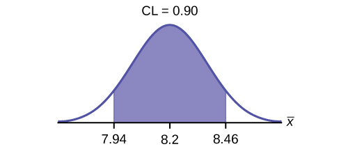
- Solution: EBM = 0.26
e. If the Census wants to increase its level of confidence and keep the error bound the same by taking another survey, what changes should it make?
f. If the Census did another survey, kept the error bound the same, and surveyed only 50 people instead of 200, what would happen to the level of confidence? Why?
- Solution: The level of confidence would decrease because decreasing n makes the confidence interval wider, so at the same error bound, the confidence level decreases.
g. Suppose the Census needed to be 98% confident of the population mean length of time. Would the Census have to survey more people? Why or why not?
5. A sample of 20 heads of lettuce was selected. Assume that the population distribution of head weight is normal. The weight of each head of lettuce was then recorded. The mean weight was 2.2 pounds with a standard deviation of 0.1 pounds. The population standard deviation is known to be 0.2 pounds.
a. Identify the following:
- = ______
- σ = ______
- n = ______
Solutions:
- = 2.2
- σ = 0.2
- n = 20
b. In words, define the random variable X.
c. In words, define the random variable .
- Solution: is the mean weight of a sample of 20 heads of lettuce.
d. Which distribution should you use for this problem?
e. Construct a 90% confidence interval for the population mean weight of the heads of lettuce. State the confidence interval, sketch the graph, and calculate the error bound.
- Solution: EBM = 0.07
- Solution: CI: (2.1264, 2.2736)
f. Construct a 95% confidence interval for the population mean weight of the heads of lettuce. State the confidence interval, sketch the graph, and calculate the error bound.
g. In complete sentences, explain why the confidence interval in F is larger than in E.
- Solution: The interval is greater because the level of confidence increased. If the only change made in the analysis is a change in confidence level, then all we are doing is changing how much area is being calculated for the normal distribution. Therefore, a larger confidence level results in larger areas and larger intervals.
h. In complete sentences, give an interpretation of what the interval in E means.
i. What would happen if 40 heads of lettuce were sampled instead of 20, and the error bound remained the same?
- Solution: The confidence level would increase.
j. What would happen if 40 heads of lettuce were sampled instead of 20, and the confidence level remained the same?
6. The mean age for all Foothill College students for a recent Fall term was 33.2. The population standard deviation has been pretty consistent at 15. Suppose that twenty-five Winter students were randomly selected. The mean age for the sample was 30.4. We are interested in the true mean age for Winter Foothill College students.[10] Let X = the age of a Winter Foothill College student.
a. = _____
- Solution: 30.4
b. n = _____
c. ________ = 15
- Solution: σ
d. In words, define the random variable .
e. What is estimating?
- Solution: μ
f. Is  known?
g. As a result of your answer to E, state the exact distribution to use when calculating the confidence interval.
- Solution: normal
h. Construct a 95% Confidence Interval for the true mean age of Winter Foothill College students by working out then answering the next seven bullet points.
- How much area is in both tails (combined)? α =________
- How much area is in each tail?
 =________
-
- Solution: 0.025
- Identify the following specifications:
-
- lower limit
- upper limit
- error bound
- The 95% confidence interval is:__________________.
-
- Solution: (24.52,36.28)
- Fill in the blanks on the graph with the areas, upper and lower limits of the confidence interval, and the sample mean.
- In one complete sentence, explain what the interval means.
-
- Solution: We are 95% confident that the true mean age for Winger Foothill College students is between 24.52 and 36.28.
- Using the same mean, standard deviation, and level of confidence, suppose that n were 69 instead of 25. Would the error bound become larger or smaller? How do you know?
- Using the same mean, standard deviation, and sample size, how would the error bound change if the confidence level were reduced to 90%? Why?
-
- Solution: The error bound for the mean would decrease because as the CL decreases, you need less area under the normal curve (which translates into a smaller interval) to capture the true population mean.
7. Among various ethnic groups, the standard deviation of heights is known to be approximately three inches. We wish to construct a 95% confidence interval for the mean height of male Swedes. Forty-eight male Swedes are surveyed. The sample mean is 71 inches. The sample standard deviation is 2.8 inches.
a. =________
b. σ =________
c. n =________
d. In words, define the random variables X and .
e. Which distribution should you use for this problem? Explain your choice.
f. Construct a 95% confidence interval for the population mean height of male Swedes.
-
- State the confidence interval.
- Sketch the graph.
- Calculate the error bound.
g. What will happen to the level of confidence obtained if 1,000 male Swedes are surveyed instead of 48? Why?
-
- 71
- 3
- 48
Solutions:
- X is the height of a Swiss male, and is the mean height from a sample of 48 Swiss males.
- Normal. We know the standard deviation for the population, and the sample size is greater than 30.
- CI: (70.151, 71.49)
-
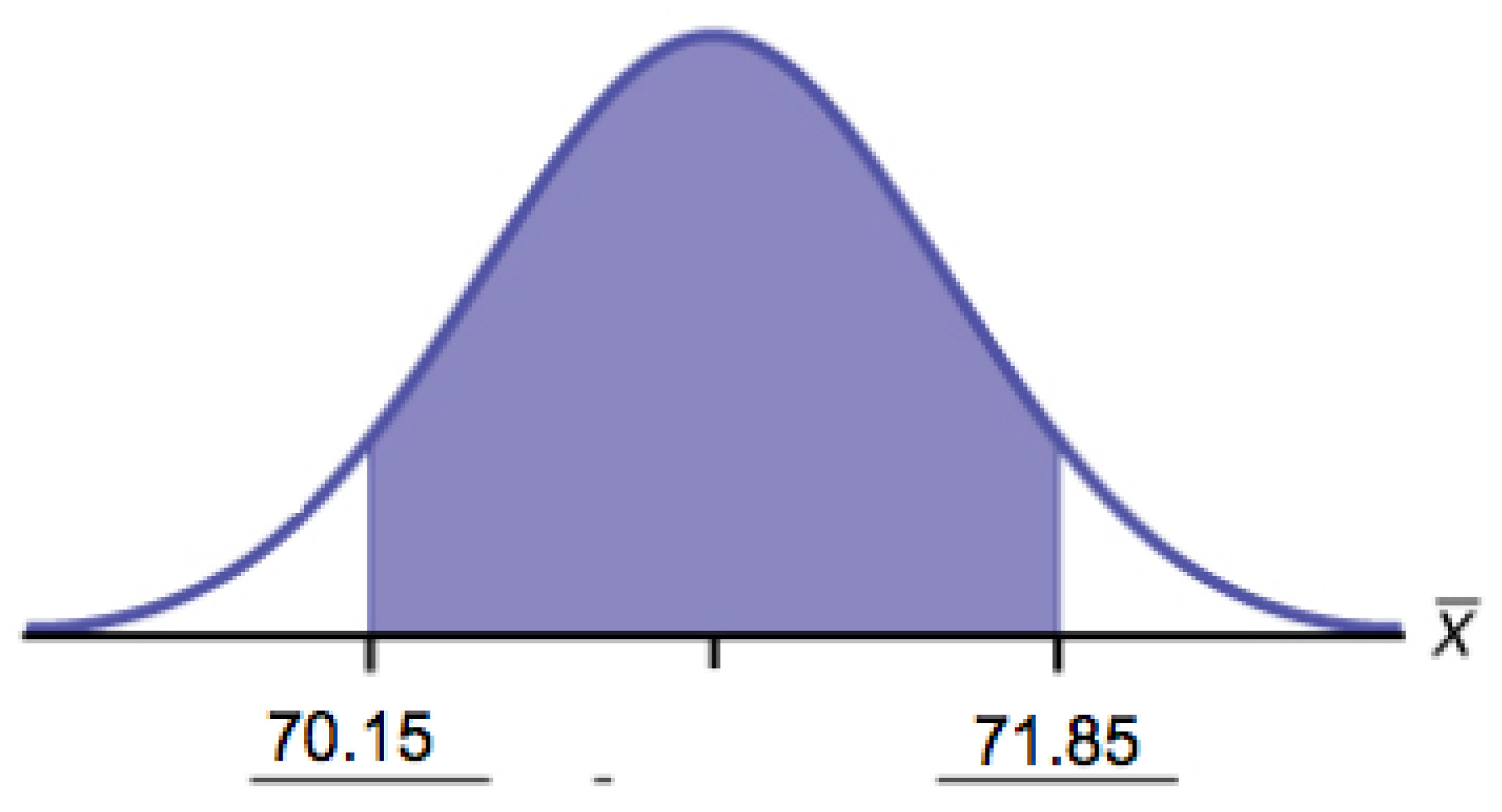
Figure 6.26 - EBM = 0.849
- The confidence interval will decrease in size, because the sample size increased. Recall, when all factors remain unchanged, an increase in sample size decreases variability. Thus, we do not need as large an interval to capture the true population mean.
8. Announcements for 84 upcoming engineering conferences were randomly picked from a stack of IEEE Spectrum magazines. The mean length of the conferences was 3.94 days, with a standard deviation of 1.28 days. Assume the underlying population is normal.
- In words, define the random variables X and .
- Which distribution should you use for this problem? Explain your choice.
- Construct a 95% confidence interval for the population mean length of engineering conferences.
- State the confidence interval.
- Sketch the graph.
- Calculate the error bound.
9. Suppose that an accounting firm does a study to determine the time needed to complete one person’s tax forms. It randomly surveys 100 people. The sample mean is 23.6 hours. There is a known standard deviation of 7.0 hours. The population distribution is assumed to be normal.
-
- =________
- σ =________
- n =________
- In words, define the random variables X and .
- Which distribution should you use for this problem? Explain your choice.
- Construct a 90% confidence interval for the population mean time to complete the tax forms.
- State the confidence interval.
- Sketch the graph.
- Calculate the error bound.
- If the firm wished to increase its level of confidence and keep the error bound the same by taking another survey, what changes should it make?
- If the firm did another survey, kept the error bound the same, and only surveyed 49 people, what would happen to the level of confidence? Why?
- Suppose that the firm decided that it needed to be at least 96% confident of the population mean length of time to within one hour. How would the number of people the firm surveys change? Why?
Solutions:
-
- = 23.6
 = 7
= 7- n = 100
- X is the time needed to complete an individual tax form. is the mean time to complete tax forms from a sample of 100 customers.
 because we know sigma.
- (22.228, 24.972)
-
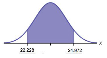
Figure 6.27 - EBM = 1.372
- It will need to change the sample size. The firm needs to determine what the confidence level should be, then apply the error bound formula to determine the necessary sample size.
- The confidence level would increase as a result of a larger interval. Smaller sample sizes result in more variability. To capture the true population mean, we need to have a larger interval.
- According to the error bound formula, the firm needs to survey 206 people. Since we increase the confidence level, we need to increase either our error bound or the sample size.
10. A sample of 16 small bags of the same brand of candies was selected. Assume that the population distribution of bag weights is normal. The weight of each bag was then recorded. The mean weight was two ounces with a standard deviation of 0.12 ounces. The population standard deviation is known to be 0.1 ounce.
-
- =________
- σ =________
- sx =________
- In words, define the random variable X.
- In words, define the random variable .
- Which distribution should you use for this problem? Explain your choice.
- Construct a 90% confidence interval for the population mean weight of the candies.
- State the confidence interval.
- Sketch the graph.
- Calculate the error bound.
- Construct a 98% confidence interval for the population mean weight of the candies.
- State the confidence interval.
- Sketch the graph.
- Calculate the error bound.
- In complete sentences, explain why the confidence interval in part f is larger than the confidence interval in part e.
- In complete sentences, give an interpretation of what the interval in part f means.
11. A camp director is interested in the mean number of letters each child sends during his or her camp session. The population standard deviation is known to be 2.5. A survey of 20 campers is taken. The mean from the sample is 7.9 with a sample standard deviation of 2.8.
-
- =________
- σ =________
- n =________
- Define the random variables X and in words.
- Which distribution should you use for this problem? Explain your choice.
- Construct a 90% confidence interval for the population mean number of letters campers send home.
- State the confidence interval.
- Sketch the graph.
- Calculate the error bound.
- What will happen to the error bound and confidence interval if 500 campers are surveyed? Why?
Solutions:
-
- 7.9
- 2.5
- 20
- X is the number of letters a single camper will send home. is the mean number of letters sent home from a sample of 20 campers.
-
N

- CI: (6.98, 8.82)
-
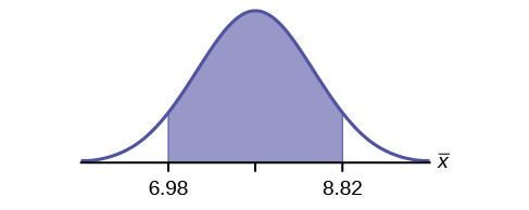
Figure 6.28 - EBM: 0.92
- The error bound and confidence interval will decrease.
12. What is meant by the term “90% confident” when constructing a confidence interval for a mean?
- If we took repeated samples, approximately 90% of the samples would produce the same confidence interval.
- If we took repeated samples, approximately 90% of the confidence intervals calculated from those samples would contain the sample mean.
- If we took repeated samples, approximately 90% of the confidence intervals calculated from those samples would contain the true value of the population mean.
- If we took repeated samples, the sample mean would equal the population mean in approximately 90% of the samples.
13. The Federal Election Commission collects information about campaign contributions and disbursements for candidates and political committees each election cycle. During the 2012 campaign season, there were 1,619 candidates for the House of Representatives across the United States who received contributions from individuals. The figure below shows the total receipts from individuals for a random selection of 40 House candidates rounded to the nearest $100. The standard deviation for this data to the nearest hundred is σ = $909,200.
| $3,600 | $1,243,900 | $10,900 | $385,200 | $581,500 |
| $7,400 | $2,900 | $400 | $3,714,500 | $632,500 |
| $391,000 | $467,400 | $56,800 | $5,800 | $405,200 |
| $733,200 | $8,000 | $468,700 | $75,200 | $41,000 |
| $13,300 | $9,500 | $953,800 | $1,113,500 | $1,109,300 |
| $353,900 | $986,100 | $88,600 | $378,200 | $13,200 |
| $3,800 | $745,100 | $5,800 | $3,072,100 | $1,626,700 |
| $512,900 | $2,309,200 | $6,600 | $202,400 | $15,800 |
- Find the point estimate for the population mean.
- Using 95% confidence, calculate the error bound.
- Create a 95% confidence interval for the mean total individual contributions.
- Interpret the confidence interval in the context of the problem.
Solution:
- = $568,873
- CL = 0.95 α = 1 – 0.95 = 0.05 = 1.96
EBM = = 1.96
  = $281,764
 - − EBM = 568,873 − 281,764 = 287,109
+ EBM = 568,873 + 281,764 = 850,637 - We estimate with 95% confidence that the mean amount of contributions received from all individuals by House candidates is between $287,109 and $850,637.
6.4 Behavior of Confidence Intervals
1. Refer back to the pizza-delivery exercise:
“Suppose average pizza delivery times are normally distributed with an unknown population mean and a population standard deviation of 6 minutes. A random sample of 28 pizza delivery restaurants is taken and has a sample mean delivery time of 36 min.”
The population standard deviation is six minutes and the sample mean deliver time is 36 minutes. Use a sample size of 20. Find a 95% confidence interval estimate for the true mean pizza delivery time.
2. Suppose we change the original problem in the pizza-delivery exercise to see what happens to the error bound if the sample size is changed. Leave everything the same except the sample size. Use the original 90% confidence level. What happens to the error bound and the confidence interval if we increase the sample size and use n = 100 instead of n = 36? What happens if we decrease the sample size to n = 25 instead of n = 36?
- = 68
- EBM =

- σ = 3; The confidence level is 90% (CL=0.90); = z0.05 = 1.645.
Solution A: If we increase the sample size n to 100, we decrease the error bound.
When n = 100: EBM = = (1.645) = 0.4935.
Solution B: If we decrease the sample size n to 25, we increase the error bound.
When n = 25: EBM = = (1.645) = 0.987.
- Increasing the sample size causes the error bound to decrease, making the confidence interval narrower.
- Decreasing the sample size causes the error bound to increase, making the confidence interval wider
6.5 Intro to Hypothesis Tests
1. When do you reject the null hypothesis?
2. The probability of winning the grand prize at a particular carnival game is 0.005. Is the outcome of winning very likely or very unlikely?
- Solution: The outcome of winning is very unlikely.
3. The probability of winning the grand prize at a particular carnival game is 0.005. Michele wins the grand prize. Is this considered a rare or common event? Why?
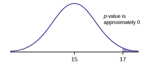
4. It is believed that the mean height of high school students who play basketball on the school team is 73 inches with a standard deviation of 1.8 inches. A random sample of 40 players is chosen. The sample mean was 71 inches, and the sample standard deviation was 1.5 years. Do the data support the claim that the mean height is less than 73 inches? The p-value is almost zero. State the null and alternative hypotheses and interpret the p-value.
H0: μ > = 73
Ha: μ < 73
The p-value is almost zero, which means there is sufficient data to conclude that the mean height of high school students who play basketball on the school team is less than 73 inches at the 5% level. The data do support the claim.
5. The mean age of graduate students at a University is at most 31 years with a standard deviation of two years. A random sample of 15 graduate students is taken. The sample mean is 32 years and the sample standard deviation is three years. Are the data significant at the 1% level? The p-value is 0.0264. State the null and alternative hypotheses and interpret the p-value.
6. Does the shaded region represent a low or a high p-value compared to a level of significance of 1%?
- Solution: The shaded region shows a low p-value.
7. What should you do when α > p-value?
8. What should you do if α = p-value?
- Solution: Do not reject H0.
9. If you do not reject the null hypothesis, then it must be true. Is this statement correct? State why or why not in complete sentences.
10. Suppose that a recent article stated that the mean time spent in jail by a first-time convicted burglar is 2.5 years. A study was then done to see if the mean time has increased in the new century. A random sample of 26 first-time convicted burglars in a recent year was picked. The mean length of time in jail from the survey was three years with a standard deviation of 1.8 years. Suppose that it is somehow known that the population standard deviation is 1.5. Conduct a hypothesis test to determine if the mean length of jail time has increased. Assume the distribution of the jail times is approximately normal.
a. Is this a test of means or proportions?
- means
b. What symbol represents the random variable for this test?
c. In words, define the random variable for this test.
- the mean time spent in jail for 26 first time convicted burglars
d. Is σ known and, if so, what is it?
e. Calculate the following:
- _______
- σ _______
- sx _______
- n _______
- 3
- 1.5
- 1.8
- 26
f. Since both σ and  are given, which should be used? In one to two complete sentences, explain why.
g. State the distribution to use for the hypothesis test.

11. A random survey of 75 death row inmates revealed that the mean length of time on death row is 17.4 years with a standard deviation of 6.3 years. Conduct a hypothesis test to determine if the population mean time on death row could likely be 15 years.
- Is this a test of one mean or proportion?
- State the null and alternative hypotheses.
H0: ____________________ Ha : ____________________ - Is this a right-tailed, left-tailed, or two-tailed test?
- What symbol represents the random variable for this test?
- In words, define the random variable for this test.
- Is the population standard deviation known and, if so, what is it?
- Calculate the following:
- = _____________
- s = ____________
- n = ____________
- Which test should be used?
- State the distribution to use for the hypothesis test.
- Find the p-value.
- At a pre-conceived α = 0.05, what is your:
- Decision:
- Reason for the decision:
- Conclusion (write out in a complete sentence):
12. The National Institute of Mental Health published an article stating that in any one-year period, approximately 9.5 percent of American adults suffer from depression or a depressive illness.[11] Suppose that in a survey of 100 people in a certain town, seven of them suffered from depression or a depressive illness. Conduct a hypothesis test to determine if the true proportion of people in that town suffering from depression or a depressive illness is lower than the percent in the general adult American population.
- Is this a test of one mean or proportion?
- State the null and alternative hypotheses.
H0: ____________________ Ha: ____________________ - Is this a right-tailed, left-tailed, or two-tailed test?
- What symbol represents the random variable for this test?
- In words, define the random variable for this test.
- Calculate the following:
- x = ________________
- n = ________________
 = _____________
- Calculate σx = __________. Show the formula set-up.
- State the distribution to use for the hypothesis test.
- Find the p-value.
- At a pre-conceived α = 0.05, what is your:
- Decision:
- Reason for the decision:
- Conclusion (write out in a complete sentence):
- H0: μ __ 66
- Ha: μ __ 66
14. We want to test if college students take less than five years to graduate from college, on the average. The null and alternative hypotheses are:
H0: μ ≥ 5
Ha: μ < 5
- H0: μ __ 45
- Ha: μ __ 45
16. In an issue of U. S. News and World Report, an article on school standards stated that about half of all students in France, Germany, and Israel take advanced placement exams and a third pass. The same article stated that 6.6% of U.S. students take advanced placement exams and 4.4% pass. Test if the percentage of U.S. students who take advanced placement exams is more than 6.6%. State the null and alternative hypotheses.
H0: p ≤ 0.066
Ha: p > 0.066
- H0: p __ 0.40
- Ha: p __ 0.40
18. You are testing that the mean speed of your cable Internet connection is more than three Megabits per second. What is the random variable? Describe in words.
- The random variable is the mean Internet speed in Megabits per second.
19. You are testing that the mean speed of your cable Internet connection is more than three Megabits per second. State the null and alternative hypotheses.
20. The American family has an average of two children. What is the random variable? Describe in words.
- The random variable is the mean number of children an American family has.
21. The mean entry level salary of an employee at a company is $58,000. You believe it is higher for IT professionals in the company. State the null and alternative hypotheses.
22. A sociologist claims the probability that a person picked at random in Times Square in New York City is visiting the area is 0.83. You want to test to see if the proportion is actually less. What is the random variable? Describe in words.
- The random variable is the proportion of people picked at random in Times Square visiting the city.
23. A sociologist claims the probability that a person picked at random in Times Square in New York City is visiting the area is 0.83. You want to test to see if the claim is correct. State the null and alternative hypotheses.
24. In a population of fish, approximately 42% are female. A test is conducted to see if, in fact, the proportion is less. State the null and alternative hypotheses.
- H0: p = 0.42
- Ha: p < 0.42
25. Suppose that a recent article stated that the mean time spent in jail by a first–time convicted burglar is 2.5 years. A study was then done to see if the mean time has increased in the new century. A random sample of 26 first-time convicted burglars in a recent year was picked. The mean length of time in jail from the survey was 3 years with a standard deviation of 1.8 years. Suppose that it is somehow known that the population standard deviation is 1.5. If you were conducting a hypothesis test to determine if the mean length of jail time has increased, what would the null and alternative hypotheses be? The distribution of the population is normal.
- H0: ________
- Ha: ________
26. A random survey of 75 death row inmates revealed that the mean length of time on death row is 17.4 years with a standard deviation of 6.3 years. If you were conducting a hypothesis test to determine if the population mean time on death row could likely be 15 years, what would the null and alternative hypotheses be?
- H0: __________
- Ha: __________
Solutions:
- H0: μ = 15
- Ha: μ ≠ 15
27. The National Institute of Mental Health published an article stating that in any one-year period, approximately 9.5 percent of American adults suffer from depression or a depressive illness.[12] Suppose that in a survey of 100 people in a certain town, seven of them suffered from depression or a depressive illness. If you were conducting a hypothesis test to determine if the true proportion of people in that town suffering from depression or a depressive illness is lower than the percent in the general adult American population, what would the null and alternative hypotheses be?
- H0: ________
- Ha: ________
28. Some of the following statements refer to the null hypothesis, some to the alternate hypothesis. State the null hypothesis, H0, and the alternative hypothesis. Ha, in terms of the appropriate parameter (μ or p).
- The mean number of years Americans work before retiring is 34.
- At most 60% of Americans vote in presidential elections.
- The mean starting salary for San Jose State University graduates is at least $100,000 per year.
- Twenty-nine percent of high school seniors get drunk each month.
- Fewer than 5% of adults ride the bus to work in Los Angeles.
- The mean number of cars a person owns in her lifetime is not more than ten.
- About half of Americans prefer to live away from cities, given the choice.
- Europeans have a mean paid vacation each year of six weeks.
- The chance of developing breast cancer is under 11% for women.
- Private universities’ mean tuition cost is more than $20,000 per year.
Solutions:
- H0: μ = 34; Ha: μ ≠ 34
- H0: p ≤ 0.60; Ha: p > 0.60
- H0: μ ≥ 100,000; Ha: μ < 100,000
- H0: p = 0.29; Ha: p ≠ 0.29
- H0: p = 0.05; Ha: p < 0.05
- H0: μ ≤ 10; Ha: μ > 10
- H0: p = 0.50; Ha: p ≠ 0.50
- H0: μ = 6; Ha: μ ≠ 6
- H0: p ≥ 0.11; Ha: p < 0.11
- H0: μ ≤ 20,000; Ha: μ > 20,000
29. Over the past few decades, public health officials have examined the link between weight concerns and teen girls’ smoking. Researchers surveyed a group of 273 randomly selected teen girls living in Massachusetts (between 12 and 15 years old). After four years the girls were surveyed again. Sixty-three said they smoked to stay thin. Is there good evidence that more than thirty percent of the teen girls smoke to stay thin? The alternative hypothesis is:
- p < 0.30
- p ≤ 0.30
- p ≥ 0.30
- p > 0.30
30. A statistics instructor believes that fewer than 20% of Evergreen Valley College (EVC) students attended the opening night midnight showing of the latest Harry Potter movie. She surveys 84 of her students and finds that 11 attended the midnight showing. An appropriate alternative hypothesis is:
- p = 0.20
- p > 0.20
- p < 0.20
- p ≤ 0.20
Solution: c
31. Previously, an organization reported that teenagers spent 4.5 hours per week, on average, on the phone. The organization thinks that, currently, the mean is higher. Fifteen randomly chosen teenagers were asked how many hours per week they spend on the phone. The sample mean was 4.75 hours with a sample standard deviation of 2.0. Conduct a hypothesis test. The null and alternative hypotheses are:
- Ho: = 4.5, Ha : > 4.5
- Ho: μ ≥ 4.5, Ha: μ < 4.5
- Ho: μ = 4.75, Ha: μ > 4.75
- Ho: μ = 4.5, Ha: μ > 4.5
6.6 Hypothesis Tests in Depth
1. Suppose the null hypothesis, H0, is: The victim of an automobile accident is alive when he arrives at the emergency room of a hospital.
Type I error: The emergency crew thinks that the victim is dead when, in fact, the victim is alive. Type II error: The emergency crew does not know if the victim is alive when, in fact, the victim is dead.
α = probability that the emergency crew thinks the victim is dead when, in fact, he is really alive = P(Type I error). β = probability that the emergency crew does not know if the victim is alive when, in fact, the victim is dead = P(Type II error).
Which is the error with the greater consequence?
Solution: Type I error (If the emergency crew thinks the victim is dead, they will not treat him.)
3. It’s a Boy Genetic Labs claim to be able to increase the likelihood that a pregnancy will result in a boy being born. Statisticians want to test the claim. Suppose that the null hypothesis, H0, is: It’s a Boy Genetic Labs has no effect on gender outcome.
Type I error: This results when a true null hypothesis is rejected. In the context of this scenario, we would state that we believe that It’s a Boy Genetic Labs influences the gender outcome, when in fact it has no effect. The probability of this error occurring is denoted by the Greek letter alpha, α.
Type II error: This results when we fail to reject a false null hypothesis. In context, we would state that It’s a Boy Genetic Labs does not influence the gender outcome of a pregnancy when, in fact, it does. The probability of this error occurring is denoted by the Greek letter beta, β.
What is the error of greater consequence?
Solution: Type I error (couples would use the It’s a Boy Genetic Labs product in hopes of increasing the chances of having a boy)
5. A certain experimental drug claims a cure rate of at least 75% for males with prostate cancer. Describe both the Type I and Type II errors in context. Which error is the more serious?
Type I: A cancer patient believes the cure rate for the drug is less than 75% when it actually is at least 75%.
Type II: A cancer patient believes the experimental drug has at least a 75% cure rate when it has a cure rate that is less than 75%.
Solution: In this scenario, the Type II error contains the more severe consequence. If a patient believes the drug works at least 75% of the time, this most likely will influence the patient’s (and doctor’s) choice about whether to use the drug as a treatment option.
Assume a null hypothesis, H0, that states the percentage of adults with jobs is at least 88%.
7. Identify the Type I and Type II errors from these four statements.
- Not to reject the null hypothesis that the percentage of adults who have jobs is at least 88% when that percentage is actually less than 88%
- Not to reject the null hypothesis that the percentage of adults who have jobs is at least 88% when the percentage is actually at least 88%.
- Reject the null hypothesis that the percentage of adults who have jobs is at least 88% when the percentage is actually at least 88%.
- Reject the null hypothesis that the percentage of adults who have jobs is at least 88% when that percentage is actually less than 88%.
8. The mean price of mid-sized cars in a region is $32,000. A test is conducted to see if the claim is true. State the Type I and Type II errors in complete sentences.
Solution:
Type I: The mean price of mid-sized cars is $32,000, but we conclude that it is not $32,000.
Type II: The mean price of mid-sized cars is not $32,000, but we conclude that it is $32,000.
9. A sleeping bag is tested to withstand temperatures of –15 °F. You think the bag cannot stand temperatures that low. State the Type I and Type II errors in complete sentences.
10. A group of doctors is deciding whether or not to perform an operation. Suppose the null hypothesis, H0, is: the surgical procedure will go well. State the Type I and Type II errors in complete sentences. Which is the error with the greater consequence?
Solution:
Type I: The procedure will go well, but the doctors think it will not.
Type II: The procedure will not go well, but the doctors think it will.
11. The power of a test is 0.981. What is the probability of a Type II error?
0.019
12. A group of divers is exploring an old sunken ship. Suppose the null hypothesis, H0, is: the sunken ship does not contain buried treasure. State the Type I and Type II errors in complete sentences.
13. A microbiologist is testing a water sample for E-coli. Suppose the null hypothesis, H0, is: the sample does not contain E-coli. The probability that the sample does not contain E-coli, but the microbiologist thinks it does is 0.012. The probability that the sample does contain E-coli, but the microbiologist thinks it does not is 0.002. What is the power of this test?
- 0.998
14. A microbiologist is testing a water sample for E-coli. Suppose the null hypothesis, H0, is: the sample contains E-coli. Which is the error with the greater consequence?
15. State the Type I and Type II errors in complete sentences given the following statements.
- The mean number of years Americans work before retiring is 34.
- At most 60% of Americans vote in presidential elections.
- The mean starting salary for San Jose State University graduates is at least $100,000 per year.
- Twenty-nine percent of high school seniors get drunk each month.
- Fewer than 5% of adults ride the bus to work in Los Angeles.
- The mean number of cars a person owns in his or her lifetime is not more than ten.
- About half of Americans prefer to live away from cities, given the choice.
- Europeans have a mean paid vacation each year of six weeks.
- The chance of developing breast cancer is under 11% for women.
- Private universities mean tuition cost is more than $20,000 per year.
Solutions:
- Type I error: We conclude that the mean is not 34 years, when it really is 34 years. Type II error: We conclude that the mean is 34 years, when in fact it really is not 34 years.
- Type I error: We conclude that more than 60% of Americans vote in presidential elections, when the actual percentage is at most 60%.Type II error: We conclude that at most 60% of Americans vote in presidential elections when, in fact, more than 60% do.
- Type I error: We conclude that the mean starting salary is less than $100,000, when it really is at least $100,000. Type II error: We conclude that the mean starting salary is at least $100,000 when, in fact, it is less than $100,000.
- Type I error: We conclude that the proportion of high school seniors who get drunk each month is not 29%, when it really is 29%. Type II error: We conclude that the proportion of high school seniors who get drunk each month is 29% when, in fact, it is not 29%.
- Type I error: We conclude that fewer than 5% of adults ride the bus to work in Los Angeles, when the percentage that do is really 5% or more. Type II error: We conclude that 5% or more adults ride the bus to work in Los Angeles when, in fact, fewer that 5% do.
- Type I error: We conclude that the mean number of cars a person owns in his or her lifetime is more than 10, when in reality it is not more than 10. Type II error: We conclude that the mean number of cars a person owns in his or her lifetime is not more than 10 when, in fact, it is more than 10.
- Type I error: We conclude that the proportion of Americans who prefer to live away from cities is not about half, though the actual proportion is about half. Type II error: We conclude that the proportion of Americans who prefer to live away from cities is half when, in fact, it is not half.
- Type I error: We conclude that the duration of paid vacations each year for Europeans is not six weeks, when in fact it is six weeks. Type II error: We conclude that the duration of paid vacations each year for Europeans is six weeks when, in fact, it is not.
- Type I error: We conclude that the proportion is less than 11%, when it is really at least 11%. Type II error: We conclude that the proportion of women who develop breast cancer is at least 11%, when in fact it is less than 11%.
- Type I error: We conclude that the average tuition cost at private universities is more than $20,000, though in reality it is at most $20,000. Type II error: We conclude that the average tuition cost at private universities is at most $20,000 when, in fact, it is more than $20,000.
16. For statements a-j in the previous question answer the following in complete sentences.
- State a consequence of committing a Type I error.
- State a consequence of committing a Type II error.
17. When a new drug is created, the pharmaceutical company must subject it to testing before receiving the necessary permission from the Food and Drug Administration (FDA) to market the drug. Suppose the null hypothesis is “the drug is unsafe.” What is the Type II Error?
- To conclude the drug is safe when in, fact, it is unsafe.
- Not to conclude the drug is safe when, in fact, it is safe.
- To conclude the drug is safe when, in fact, it is safe.
- Not to conclude the drug is unsafe when, in fact, it is unsafe.
Solution: b
18. A statistics instructor believes that fewer than 20% of Evergreen Valley College (EVC) students attended the opening midnight showing of the latest Harry Potter movie. She surveys 84 of her students and finds that 11 of them attended the midnight showing. The Type I error is to conclude that the percent of EVC students who attended is ________.
- at least 20%, when in fact, it is less than 20%.
- 20%, when in fact, it is 20%.
- less than 20%, when in fact, it is at least 20%.
- less than 20%, when in fact, it is less than 20%.
19. It is believed that Lake Tahoe Community College (LTCC) Intermediate Algebra students get less than seven hours of sleep per night, on average. A survey of 22 LTCC Intermediate Algebra students generated a mean of 7.24 hours with a standard deviation of 1.93 hours.[13] At a level of significance of 5%, do LTCC Intermediate Algebra students get less than seven hours of sleep per night, on average?
The Type II error is not to reject that the mean number of hours of sleep LTCC students get per night is at least seven when, in fact, the mean number of hours
- is more than seven hours.
- is at most seven hours.
- is at least seven hours.
- is less than seven hours.
Solution: d
20. Previously, an organization reported that teenagers spent 4.5 hours per week, on average, on the phone. The organization thinks that, currently, the mean is higher. Fifteen randomly chosen teenagers were asked how many hours per week they spend on the phone. The sample mean was 4.75 hours with a sample standard deviation of 2.0. Conduct a hypothesis test, the Type I error is:
- to conclude that the current mean hours per week is higher than 4.5, when in fact, it is higher
- to conclude that the current mean hours per week is higher than 4.5, when in fact, it is the same
- to conclude that the mean hours per week currently is 4.5, when in fact, it is higher
- to conclude that the mean hours per week currently is no higher than 4.5, when in fact, it is not higher
References
Image References
Figure 6.17: Figure 7.16 from OpenStax Introductory Statistics (2013) (CC BY 4.0). Retrieved from https://openstax.org/books/introductory-statistics/pages/7-practice
Figure 6.18: Figure 7.17 from OpenStax Introductory Statistics (2013) (CC BY 4.0). Retrieved from https://openstax.org/books/introductory-statistics/pages/7-practice
Figure 6.19: Figure 7.17 from OpenStax Introductory Statistics (2013) (CC BY 4.0). Retrieved from https://openstax.org/books/introductory-statistics/pages/7-practice
Figure 6.21: Figure 8.4 from OpenStax Introductory Statistics (2013) (CC BY 4.0). Retrieved from https://openstax.org/books/introductory-statistics/pages/8-1-a-single-population-mean-using-the-normal-distribution
Figure 6.23: Figure 8.12 from OpenStax Introductory Statistics (2013) (CC BY 4.0). Retrieved from https://openstax.org/books/statistics/pages/8-solutions#eip-773-solution
Figure 6.24: Figure 8.13 from OpenStax Introductory Statistics (2013) (CC BY 4.0). Retrieved from https://openstax.org/books/statistics/pages/8-solutions#eip-773-solution
Figure 6.25: Figure from Lumen Learning Introduction to Statistics (CC BY 4.0). Retrieved from https://courses.lumenlearning.com/introstats1/chapter/section-exercises-7/
Figure 6.26: Figure 8.18 from OpenStax Introductory Statistics (2013) (CC BY 4.0). Retrieved from https://openstax.org/books/statistics/pages/8-solutions#eip-773-solution
Figure 6.27: Figure 8.19 from OpenStax Introductory Statistics (2013) (CC BY 4.0). Retrieved from https://openstax.org/books/statistics/pages/8-solutions#eip-773-solution
Figure 6.28: Figure 8.20 from OpenStax Introductory Statistics (2013) (CC BY 4.0). Retrieved from https://openstax.org/books/statistics/pages/8-solutions#eip-773-solution
Figure 6.30: Figure 9.24 from OpenStax Introductory Statistics (2013) (CC BY 4.0). Retrieved from https://openstax.org/books/introductory-statistics/pages/9-practice
Text
Baran, Daya. “20 Percent of Americans Have Never Used Email.” WebGuild, 2010. Available online at http://www.webguild.org/20080519/20-percent-of-americans-have-never-used-email (accessed May 17, 2013).
Data from The Flurry Blog, 2013. Available online at http://blog.flurry.com (accessed May 17, 2013).
Data from the United States Department of Agriculture.
Image credit: comedy_nose/flickr
“American Fact Finder.” U.S. Census Bureau. Available online at http://factfinder2.census.gov/faces/nav/jsf/pages/searchresults.xhtml?refresh=t (accessed July 2, 2013).
“Disclosure Data Catalog: Candidate Summary Report 2012.” U.S. Federal Election Commission. Available online at http://www.fec.gov/data/index.jsp (accessed July 2, 2013).
“Headcount Enrollment Trends by Student Demographics Ten-Year Fall Trends to Most Recently Completed Fall.” Foothill De Anza Community College District. Available online at http://research.fhda.edu/factbook/FH_Demo_Trends/FoothillDemographicTrends.htm (accessed September 30,2013).
Kuczmarski, Robert J., Cynthia L. Ogden, Shumei S. Guo, Laurence M. Grummer-Strawn, Katherine M. Flegal, Zuguo Mei, Rong Wei, Lester R. Curtin, Alex F. Roche, Clifford L. Johnson. “2000 CDC Growth Charts for the United States: Methods and Development.” Centers for Disease Control and Prevention. Available online at http://www.cdc.gov/growthcharts/2000growthchart-us.pdf (accessed July 2, 2013).
La, Lynn, Kent German. “Cell Phone Radiation Levels.” c|net part of CBX Interactive Inc. Available online at http://reviews.cnet.com/cell-phone-radiation-levels/ (accessed July 2, 2013).
“Mean Income in the Past 12 Months (in 2011 Inflaction-Adjusted Dollars): 2011 American Community Survey 1-Year Estimates.” American Fact Finder, U.S. Census Bureau. Available online at http://factfinder2.census.gov/faces/tableservices/jsf/pages/productview.xhtml?pid=ACS_11_1YR_S1902&prodType=table (accessed July 2, 2013).
“Metadata Description of Candidate Summary File.” U.S. Federal Election Commission. Available online at http://www.fec.gov/finance/disclosure/metadata/metadataforcandidatesummary.shtml (accessed July 2, 2013).
“National Health and Nutrition Examination Survey.” Centers for Disease Control and Prevention. Available online at http://www.cdc.gov/nchs/nhanes.htm (accessed July 2, 2013).
(Credit: Robert Neff)
Data from the National Institute of Mental Health. Available online at http://www.nimh.nih.gov/publicat/depression.cfm.
- La, Lynn, Kent German. "Cell Phone Radiation Levels." part of CBX Interactive Inc. Available online at http://reviews.cnet.com/cell-phone-radiation-levels/ (accessed July 2, 2013). ↵
- “2012 College-Bound Seniors Total Group Profile Report.” CollegeBoard, 2012. Available online at http://media.collegeboard.com/digitalServices/pdf/research/TotalGroup-2012.pdf (accessed May 14, 2013). ↵
- Data from The Flurry Blog, 2013. Available online at http://blog.flurry.com (accessed May 17, 2013). ↵
- Data from The Flurry Blog, 2013. Available online at http://blog.flurry.com (accessed May 17, 2013). ↵
- Data from the United States Department of Agriculture. ↵
- “National Health and Nutrition Examination Survey.” Center for Disease Control and Prevention. Available online at http://www.cdc.gov/nchs/nhanes.htm (accessed May 17, 2013). ↵
- La, Lynn, Kent German. "Cell Phone Radiation Levels." part of CBX Interactive Inc. Available online at http://reviews.cnet.com/cell-phone-radiation-levels/ (accessed July 2, 2013). ↵
- La, Lynn, Kent German. "Cell Phone Radiation Levels." part of CBX Interactive Inc. Available online at http://reviews.cnet.com/cell-phone-radiation-levels/ (accessed July 2, 2013). ↵
- “American Fact Finder.” U.S. Census Bureau. Available online at http://factfinder2.census.gov/faces/nav/jsf/pages/ searchresults.xhtml?refresh=t (accessed July 2, 2013). ↵
- “Headcount Enrollment Trends by Student Demographics Ten-Year Fall Trends to Most Recently Completed Fall.” Foothill De Anza Community College District. Available online at http://research.fhda.edu/factbook/FH_Demo_Trends/ FoothillDemographicTrends.htm (accessed September 30,2013). ↵
- Data from the National Institute of Mental Health. Available online at http://www.nimh.nih.gov/publicat/depression.cfm. ↵
- Data from the National Institute of Mental Health. Available online at http://www.nimh.nih.gov/publicat/depression.cfm. ↵
- King, Bill.“Graphically Speaking.” Institutional Research, Lake Tahoe Community College. Available online at http://www.ltcc.edu/web/about/institutional-research (accessed April 3, 2013). ↵
Using information from a sample to answer a question, or generalize, about a population
A subset of the population studied
The whole group of individuals who can be studied to answer a research question
Using sample data to calculate a single statistic as an estimate of an unknown population parameter
A decision making procedure for determining whether sample evidence supports a hypothesis
The value that is calculated from a sample used to estimate an unknown population parameter
A number that is used to represent a population characteristic and can only be calculated as the result of a census
A number calculated from a sample
The idea that samples from the same population can yield different results
The probability distribution of a statistic at a given sample size
As the number of trials in a probability experiment increases, the relative frequency of an event approaches the theoretical probability
The standard deviation of a sampling distribution
States that if there is a population with mean μ and standard deviation σ and you take sufficiently large random samples from the population, then the distribution of the sample means will be approximately normally distributed
The facet of statistics dealing with using a sample to generalize (or infer) about the population
An interval built around a point estimate for an unknown population parameter
Roughly 68% of values are within 1 standard deviation of the mean, roughly 95% of values are within 2 standard deviations of the mean, and 99.7% of values are within 3 standard deviations of the mean
How much a point estimate can be expected to differ from the true population value; made up of the standard error multiplied by the critical value
Point that lies on a distribution that acts as a cut-off value for accepting or rejecting the null hypothesis
The claim that is assumed to be true and is tested in a hypothesis test
A working hypothesis that is contradictory to the null hypothesis
A measure of how far what you observed is from the hypothesized (or claimed) value
The probability that an event will occur, assuming the null hypothesis is true
Probability that a true null hypothesis will be rejected, also known as Type I error and denoted by α
Finding sufficient evidence that the effect we see is not just due to variability, often from rejecting the null hypothesis
The decision is to reject the null hypothesis when, in fact, the null hypothesis is true
Erroneously rejecting a true null hypothesis, or erroneously failing to reject a false null hypothesis
The probability of failing to reject a true hypothesis
