25 Chapter 25: Accuracy Assessment
Introduction
Accuracy Assessment compares a classified image to a reference image that matches the classified image with respect to scale, detail, date, categories, and projection. This is often conducted through a pixel-by-pixel comparison of a classified image to an image assumed to be a correct representation of the Earth’s surface (such as an aerial photo). An accuracy assessment is conducted to determine how well a specific classification method performed. Accuracy assessments are conducted for both unsupervised and supervised classifications and are always included in any project report. Although the pixel-by-pixel comparison assesses overall agreement between the two images, in a remote sensing context, we typically regard the reference map as an accuracy standard and report disagreements between the two images as errors.1
An accuracy assessment composes an error matrix by comparing the two images pixel-by-pixel. Mismatches are regarded as errors and are tabulated with respect to the number of incorrect matches, how the mismatched pixel was classified, and the percent of mismatched pixels. An error matrix consists of a table of values comparing the informational class code assigned to a specific pixel during the classification process to the actual informational class identified from an aerial photo. It is impossible to compare all pixels (which may number in the millions). Therefore, a randomly selected pixel sample is used to generate the error matrix. Later in this chapter, we provide an example to illustrate the calculation of the error matrix.
The final step of an accuracy assessment includes the calculation of Cohen’s kappa coefficient derived from the error matrix. Kappa tells us how well the classification process performed compared to a random assignment of values. For example, did we do better than randomly assigning the pixels to a specific informational class?
This chapter provides a step-by-step process for performing an accuracy assessment by completing an error matrix, then calculating Kappa.
The step-by-step process includes:
- Generating a set of random points in ArcGIS® Pro.
- Identifying the informational class of the pixel in an aerial photo associated with each point.
- For each of these same points, the information class assigned during the classification process is identified.
- Compiling an error matrix.
- Calculating the accuracy percentage for each informational class.
- Calculating the percentage of the producer’s accuracy, user’s accuracy, and overall accuracy.
- Calculating Kappa.
For more details on Accuracy Assessment and Kappa, see Introduction to Remote Sensing by Campbell, Wynne, and Thomas 6th, 2022 and Assessing the Accuracy of Remotely Sensed Data by Congalton & Green, 2019.
As a reminder of our informational classes:
|
Class Number |
Information Class |
Color designation |
|
1 |
Urban/built-up/transportation |
Red |
|
2 |
Mixed agriculture |
Yellow |
|
3 |
Forest & Wetland |
Green |
|
4 |
Open water |
Blue |
Classification Results from Prior Chapters
In Chapter 21, Classification of a Landsat 9 Image (Unsupervised), and Chapter 24: Conducting a Supervised Classification of a Landsat 9 Image, we calculated the number of pixels for each informational class and the percentage of the total land area represented by that class.
Figure 25.1 is the attribute table of the unsupervised classified image from Chapter 21.
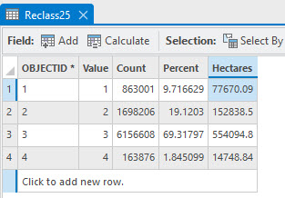
Figure 25.1 Attribute table from unsupervised classified image
Figure 25.2 is the attribute table for the maximum likelihood classified image from Chapter 24.
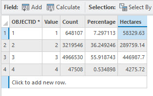
Figure 25.2 Attribute Table for the maximum likelihood classified image
Figure 25.3 is the attribute table for the Support Vector Machine (SVM) classified image from Chapter 24.
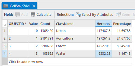
Figure 25.3 Attribute table for the SVM cell statistics classified image
Comparing the results from the three tables:
|
Information Class |
Hectares |
Percent |
||||
|
unsupervised |
supervised |
SVM |
Unsupervised |
Supervised |
SVM |
|
|
Urban |
77,670.09 |
58,329.63 |
117,487.80 |
9.72 |
7.30 |
14.70 |
|
Agriculture |
152,838.50 |
289,759.14 |
197,261.20 |
19.12 |
36.25 |
24.68 |
|
Forest |
554,094.80 |
446,987.7 |
475,270.90 |
69.32 |
55.92 |
59.46 |
|
Water |
14,748.84 |
4,475.72 |
9,332.28 |
1.85 |
0.53 |
1.17 |
The three methods generated significantly different results. Remember, we made different decisions in both chapters when performing the classifications. For Chapter 21, we chose 25 spectral classes for efficiency in demonstrating the chapter but noted that 50 classes were likely more appropriate. Which method performed best? An accuracy assessment can reveal the difference.
Setting up ArcGIS Pro for an Accuracy Assessment
Open the project created for Chapter 24 and save it with a new name, for example, Accuracy Assessment.
The only layers we need in the project are the three classified images, so remove all layers except the maximum likelihood classified image and the SVM classified image. Then add the Reclass of the unsupervised classified image created in Chapter 21. Add the World Imagery Basemap option. Set the workspaces. Set the symbology to the correct informational class values and colors if necessary (Figure 25.4).
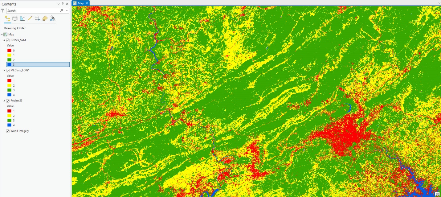
Figure 25.4 ArcGIS Pro with 3 classified images in Contents
Generating a Set of Random Points
A random points file is first generated to eliminate bias from the accuracy assessment, for example, only choosing pixels that are known to be classified correctly. Go to the Analysis tab, Tools, and search for Accuracy. Choose Create Accuracy Assessment Points (Spatial Analyst Tools) (Figure 25.5).
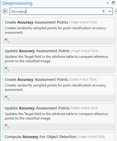
Figure 25.5 Searching for Accuracy Assessment tool
For Input Raster or Feature Class Data any of the classified images may be selected. This choice will limit the areal extent within which the random points are generated and will automatically extract the class values when the new feature class is created. We chose the maximum likelihood image.
Name the Output Accuracy Assessment Points feature class, and ensure it is saved in the geodatabase.
The Target Field is Classified.
The number of random points chosen depends on the extent of the area, the number of informational classes, and other considerations. The number of random points defaults to 500, however, for our purpose of demonstrating an accuracy assessment process, we have reduced the number of random points to 100.
Three Sampling Strategies are available. We want Random and will not choose a stratification process for this assessment. For other projects stratification might be appropriate, academic literature will need to be consulted for this decision.
Once the fields are populated, as shown in Figure 25.6, click Run.
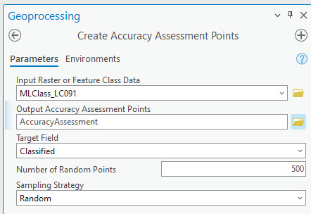
Figure 25.6 The Accuracy Assessment Points tool
This tool runs quickly. A completed message displays at the bottom of the Geoprocessing dialog box, and a new layer appears in Contents and displays in the map viewer. The symbology for the points is light green (yours may be different) and challenging to see (Figure 25.7).
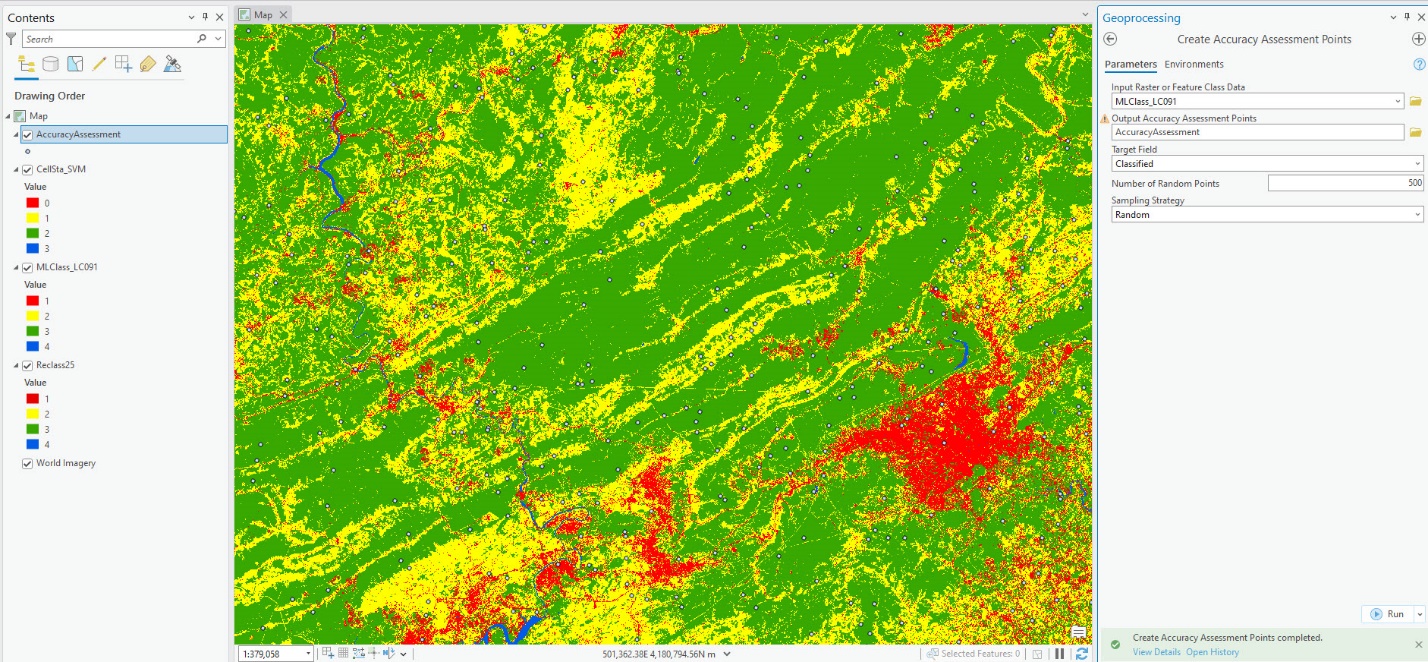
Figure 25.7 Results from the Accuracy Assessment Points tool
In Figure 25.8, we changed the symbology of the random points layer to black to enhance their visibility.
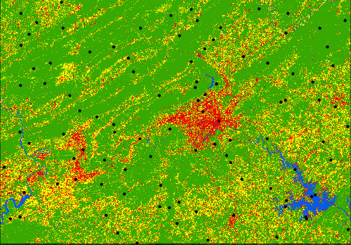
Figure 25.8 Enhancement of the individual points
Open the Attribute Table of this new point feature class (Figure 25.9).
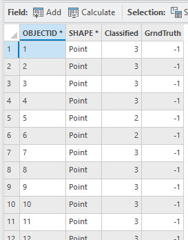
Figure 25.9 Attribute table for the accuracy assessment points feature class
The informational class values for each point were automatically extracted from the maximum likelihood classified image. A second field added is called GrndTruth. Ground truth is also known as field data in other usage. This field can be used if the true value for each of your points will be based on field evaluation.
For our purposes, we are not verifying with ground truth, so we will delete the GrndTruth field. Right-click the column and choose Delete Field (Figure 25.10).
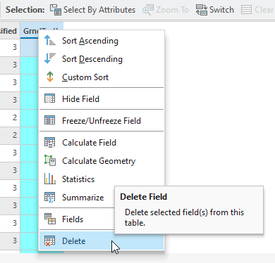
Figure 25.10 Deleting a field in the attribute table
ArcGIS® Pro asks if you are sure; select Yes.
Now add two fields to the attribute table—ML and AERIAL. Yes, maximum likelihood is already populated, but the field name says “Classified”, so we want to be clear to which image those values belong. The fields should be numeric with no decimal points (Figure 25.11).
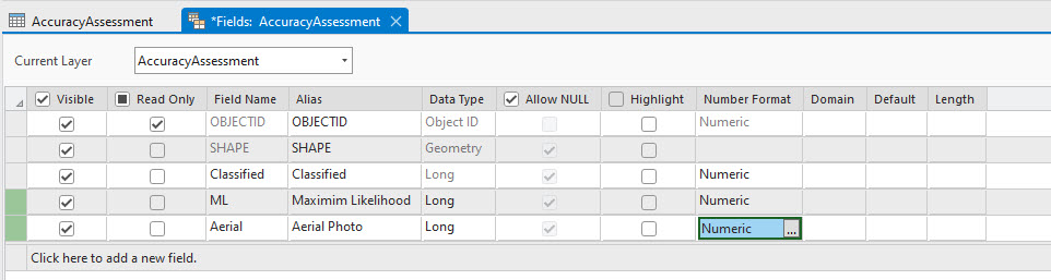
Figure 25.11 Adding new fields to the attribute table
Don’t forget to Save and close the Fields View (Figure 25.12).
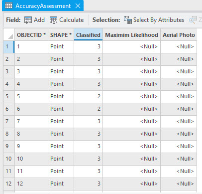
Figure 25.12 New fields added to the attribute table
Next, right-click on the Maximum Likelihood field and choose Calculate Field. In the Calculate Field dialog box, choose “Classified” for the ML= entry (Figure 25.13).
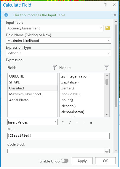
Figure 25.13 Calculating the maximum likelihood field
We will be using the Aerial Photo field, not shown in Figure 25.13, later. Next, we must populate the informational class values for the two other classified images.
Go to Tools under the Analysis tab and search for Extract Multi Values to Points (Figure 25.14) This tool was previously demonstrated in Chapter 23.
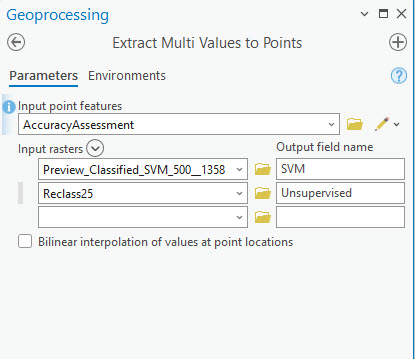
Figure 25.14 Extracting values for the other two classified images
We now have the informational class values for all three classified images in our accuracy assessment random points attribute table (Figure 25.15).
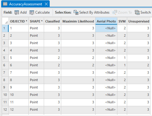
Figure 25.15 The attribute table with values for all 3 classified images
Now we will use the aerial imagery base map to populate the informational class for the Aerial Photo field. Please note that when conducting an accuracy assessment, you need to use an aerial image acquired as close to the date of the original Landsat image as possible. For example, when examining the extent of urbanization, you do not compare an aerial image from the 1970s to a Landsat image acquired in 2023.
The Aerial Photo field must be populated individually. First, make sure the only image turned on is the base map. Change the color if you cannot see the points well on the base map.
Right-click on a row in the Attribute Table and select Zoom to (Figure 25.16).
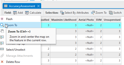
Figure 25.16 Zooming to points to identify the aerial photo point value
This zooms to the point, and we can clearly see that this is agriculture associated with Class 2 (Figure 25.17).
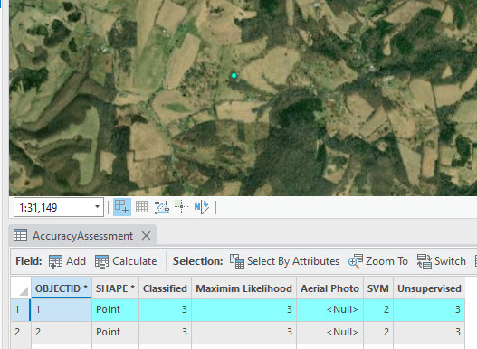
Figure 25.17 Example of an agricultural point
Double-click in the cell for the selected point under the Aerial Photo column and enter the correct information class, 2 for agriculture (Figure 25.18).
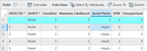
Figure 25.18 Example of adding a value to the aerial photo field associated with an agriculture point
Continue to follow this procedure for all 100 points until all points are classified based on the aerial photo. As seen in the figure below, it may be necessary to zoom out to confirm the location. Zooming in too far may make it difficult to determine if, for example, a brown pixel is a paved area or a bare agriculture field (Figure 25.19).
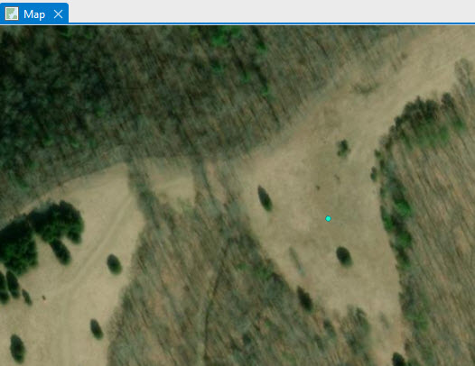
Figure 25.19 Example of a point on a field
Save frequently, both the edits and the project! To save edits, click the Save button, in the Manage Edits group of the Edit tab on the ribbon (Figure 25.20)

Figure 25.20 Location of the save button
Be sure that all 100 points are entered for Aerial Photo values.
Summarizing the Results for the Error Matrix
With the Attribute Table open, right-click on the column for Aerial Photo and select Summarize (Figure 25.21).
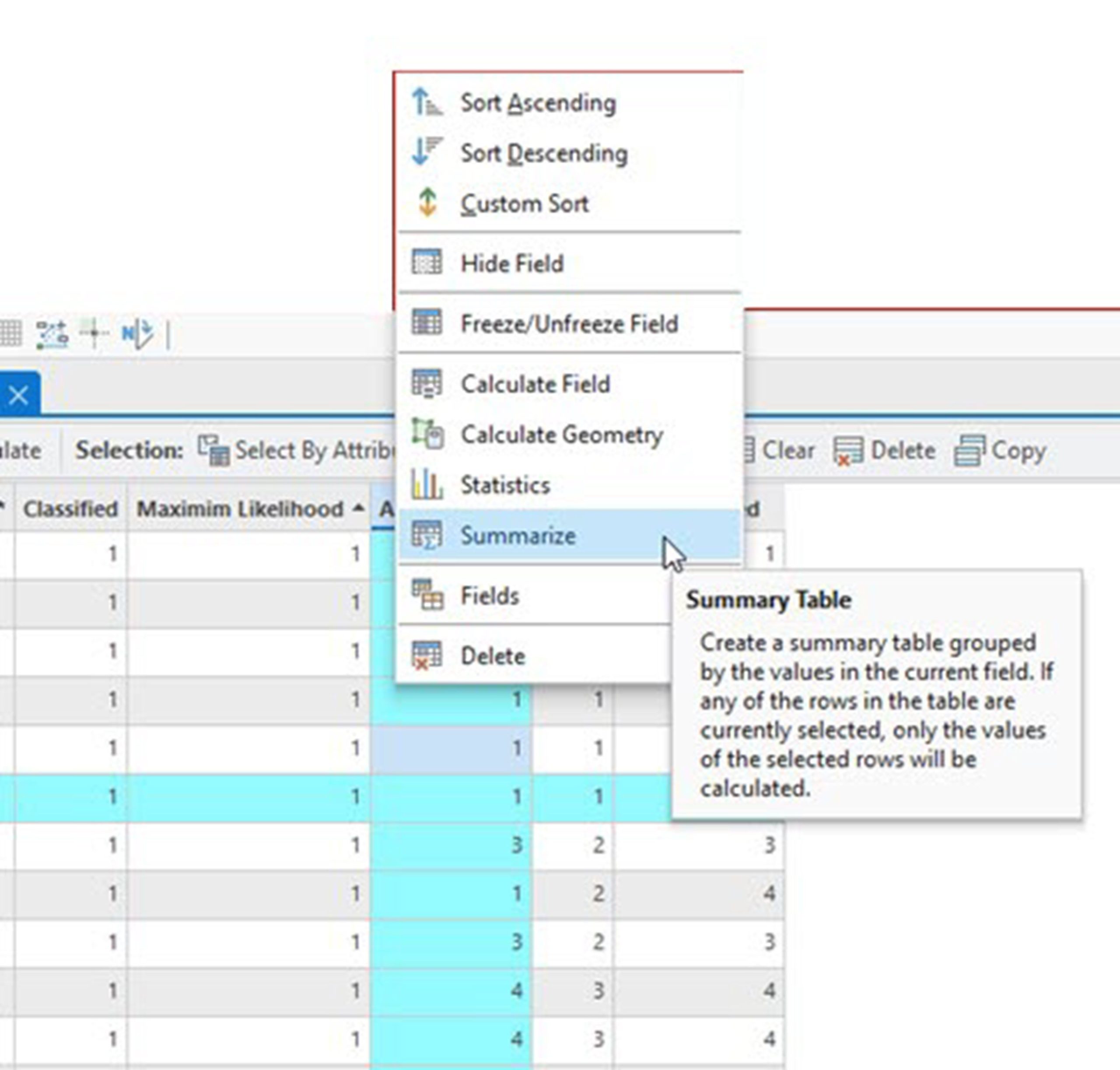
Figure 25.21 Creating a summary of the attribute table
The Summary Statistic geoprocessing window opens (Figure 25.22). Please follow the next few steps very carefully.
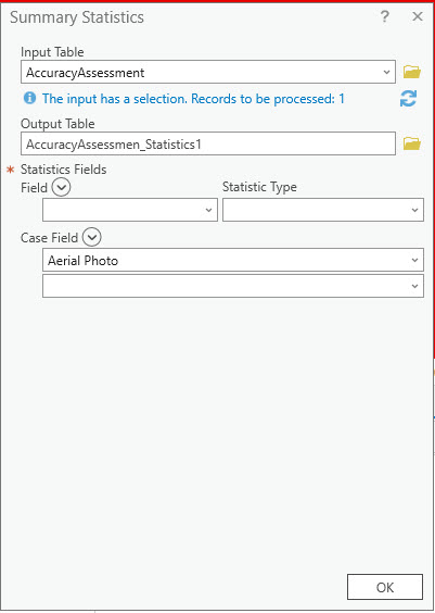
Figure 25.22 The Summary Statistics tool
We summarize class values relative to Aerial, so choose Aerial Photo for the first Statistics Field. And we want a Count of the number of pixels for each informational class (1, 2, 3, and 4). We are comparing one of the classified images (we chose the unsupervised), so it is entered in the second Statistics Field, again with Count as the statistic. Under Case field (this represents the name of the attribute column in the table), we want to list both again—Aerial Photo in the first blank and the name of the classification scheme in the second. In Figure 25.23, Aerial Photo and Maximum Likelihood are the names entered.
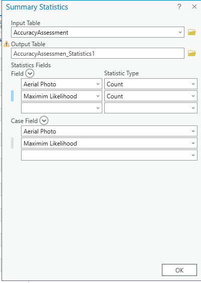
Figure 25.23 The Summary Statistics tool
Once completed as shown above, select Run. This tool runs very quickly and results in a Standalone Table in Contents.
Figure 25.24 Location of standalone tables in Contents
Right-click on the table name and open the Attribute Table. We have a summary of Aerial Photo classes and maximum likelihood classes for all 100 points (Figure 25.25).
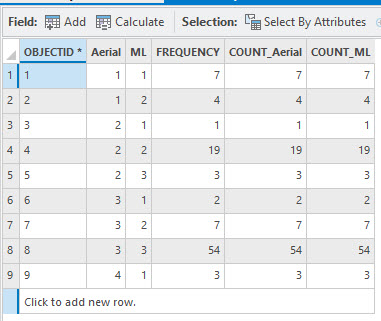
Figure 25.25 Standalone table
The following summary of the first four rows helps interpret the table:
- 1st Column: the informational class for those pixels identified from the aerial photo.
- 2nd Column: the informational class for those same pixels that are classified as such in the maximum likelihood (ML) classified image.
- 3rd – 5th Columns: the number of pixels that meet both qualifications. Please note that these counts are all the same for each column, do not add them together.
- 1st Row: 7 are identified as urban (1) in the aerial photo and urban (1) in the ML classified image.
- 2nd Row: 4 points are identified as urban (1) in the aerial photo but as agriculture (2) in the ML classified image.
- 3rd Row: 1 point is identified as agriculture (2) in the aerial photo but classified as urban (1) in the ML classified image.
- 4th Row: 19 points are identified as agriculture (2) in the aerial photo and classified as agriculture (2) in the ML classified image.
- 5th Row: 3 points are identified as agriculture (2) in the aerial photo and forest (3) in the ML classified image.
- 6th Row: 2 points are identified as forest (3) in the aerial photo and urban in the ML classified image.
- 7th Row: 7 points are identified as forest (3) in the aerial photo and agriculture (2) in the ML classified image.
- 8th Row: 54 points are identified as forest (3) in the aerial photo and forest (3) in the ML classified image.
- 9th Row: 3 points are identified as water in the aerial photo and urban in the ML classified image.
Do this same summarization for the next two columns of classified images, SVM and unsupervised. This can be done all in one table, but the table is extremely difficult to read, so it is recommended that you complete this separately for each image.
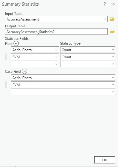
Figure 25.26 The Summary Statistics tool for the SVM classified image
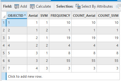
Figure 25.27 Results of SVM showing summary statistics
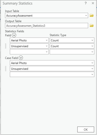
Figure 25.28 The Summary Statistics tool for the unsupervised image
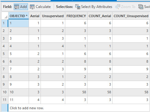
Figure 25.29 The results of the unsupervised summary statistics
Now we can compile the Error Matrix and calculate Kappa for each classification scheme.
Compiling the Error Matrix
- Remember:
|
Class Number |
Information Class |
Color designation |
|
1 |
Urban/built-up/transportation |
Red |
|
2 |
Mixed agriculture |
Yellow |
|
3 |
Forest & Wetland |
Green |
|
4 |
Open water |
Blue |
We are going to compile the matrix for the unsupervised classified image. From the tables above, the unsupervised image values were added to the random points file as Classified.
Error Matrix – Maximum Likelihood Classified Image
|
|
Water (4) |
Urban (1) |
Forest (3) |
Agriculture (2) |
Row Total |
|
Water (4) |
0 (a) |
3 (b) |
0 (c) |
0 (d) |
3 (e) |
|
Urban (1) |
0 (f) |
7 (g) |
0 (h) |
4 (i) |
11 (j) |
|
Forest (3) |
0 (k) |
2 (l) |
54 (m) |
7 (n) |
63 (o) |
|
Agriculture (2) |
0 (p) |
1 (q) |
3 (r) |
19 (s) |
23 (t) |
|
|
0 (u) |
13 (v) |
57 (w) |
30 (x) |
80 (y) |
The values in the error matrix you generate will be different from what is shown above because your random set of points will differ from our example. But we will explain each field so that you can interpret your matrix. Each field in the above error matrix contains a letter within parenthesis. We will use each letter to explain the number that belongs in that field.
a: The number of random points that were identified as water in the aerial photo and classified as water in the ML classified image
b: The number of random points that were identified as water in the aerial photo but classified as urban in the ML classified image
c: The number of random points that were identified as water in the aerial photo but were classified as forest in the ML classified image
d: The number of random points that were identified as water in the aerial photo but classified as agriculture in the ML classified image
e: Total of the Row
f: The number of random points that were identified as urban in the aerial photo but were classified as water in the ML classified image
g: The number of random points that were classified as urban in the aerial photo and urban in the ML classified image
h: The number of random points that were classified as urban in the aerial photo but forest in the ML classified image
i: The number of random points that were classified as urban in the aerial photo but agriculture in the ML classified image
j: Total of the Row
k: The number of random points that were classified as forest in the aerial photo but water in the ML classified image
l: The number of random points that were classified as forest in the aerial photo but urban in the ML classified image
m: The number of random points that were classified as forest in the aerial photo and forest in the ML classified image
n: The number of random points that were classified as forest in the aerial photo but agriculture in the ML classified image
o: Total of the Row
p: The number of random points that were classified as agriculture in the aerial photo but water in the ML classified image
q: The number of random points that were classified as agriculture in the aerial photo but urban in the ML classified image
r: The number of random points that were classified as agriculture in the aerial photo but forest in the ML classified image
s: The number of random points that were classified as agriculture in the aerial photo and agriculture in the ML classified image
t: Total of the Row
u: Total of the Column
v: Total of the Column
w: Total of the Column
x: Total of the Column
y: Sum of fields a, g, m and s
Calculating Producer’s, User’s, and Overall Accuracy
Producer’s accuracy is the percentage of random points on the ground that are classified correctly on the map from the mapmaker’s point of view. These are calculated separately for each informational class and are the number of correctly classified pixels for that image divided by the total number of ground truth points (aerial photo points) for that class.
User’s Accuracy is the percentage of a class’s random points corresponding to the number of aerial photo points. This communicates to the map users the accuracy of their point of view. It is calculated by dividing the number of correct pixels for a class by the total number of points assigned to that class.
Overall accuracy is the number of random points that are the same in both images, divided by the total number of random points. For our matrix above, that is 80 points (0 water, 7 urban, 54 forest, and 19 agriculture). We have 100 random points, so our overall accuracy is 80/100 or 80%.
Errors of omission and errors of commission can also be calculated from the error matrix. We will not discuss these specific calculations or their use in this chapter. For more information, please reference Campbell, Wynne, and Thomas’s Introduction to Remote Sensing, 6th edition, 2023.
Calculation of Cohen’s Kappa (k)
Kappa provides insight into our classification scheme and whether we achieved results better than we would have achieved strictly by chance. Kappa can range from – 1 to + 1.
The formula for kappa is:
(Observed – Expected) / (1 – Expected)
Observed is overall accuracy. Expected is calculated from the row and column totals above.
First, calculate the product of the rows and columns.
|
|
Water Column |
Urban Column |
Forest Column |
Agriculture Column |
|
Water Row |
0 x 3 = 0 |
3 x 13 = 69 |
0 x 57 = 0 |
0 x 30 = 0 |
|
Urban Row |
11 x 0 = 0 |
11 x 13 = 143 |
11 x 57 = 627 |
11 x 30 = 330 |
|
Forest Row |
63 x 0 = 0 |
63 x 13 = 819 |
63 x 57 = 3591 |
63 x 30 = 1890 |
|
Agriculture Row |
23 x 0 = 0 |
23 x 13 = 299 |
23 x 57 = 1311 |
23 x 30 = 690 |
Then calculate what would be expected based on chance:
The product matrix is the sum of the diagonals (the highlighted values): 0 + 143 + 3591 + 690 = 4424
The Cumulative Sum is: 0 + 0 + 0 + 0 + 69 + 143 + 819 + 299 + 0 + 627 + 3591 + 1311 + 0 + 330 + 1890 + 690 = 9697
So, the expected is 4424 / 9697 = 45.6%
k = (0.80-0.456) / (1 – 0.456) = 0.632 = 63.2%
The kappa coefficient for this classification is 0.632, which means the classification is 63.2% better than would have occurred strictly by chance.
Remember, we only used 100 random points to assess this classification’s accuracy. Most of the points were forest; very few water and urban points were randomly chosen. In this example, the number of random points is very low. The number should be much higher when conducting an accuracy assessment to support your research project. We used a small number of values for the accuracy assessment to illustrate the process using a practical example.
Now calculate your overall accuracy and Cohen’s kappa for your SVM and unsupervised image. To assist you with your understanding of the process, the following two tables are the calculations for our images.
Error Matrix – SVM Classified Image
|
|
Water (4) |
Urban (1) |
Forest (3) |
Agriculture (2) |
Row Totals |
|
Water (4) |
0 |
0 |
3 |
0 |
3 |
|
Urban (1) |
0 |
10 |
0 |
1 |
11 |
|
Forest (3) |
0 |
8 |
0 |
55 |
63 |
|
Agriculture (2) |
0 |
19 |
0 |
4 |
23 |
|
Column Totals |
0 |
37 |
3 |
60 |
14 |
Error Matrix – Unsupervised Classified Image
|
|
Water (4) |
Urban (1) |
Forest (3) |
Agriculture (2) |
Row totals |
|
Water (4) |
3 |
0 |
0 |
0 |
3 |
|
Urban (1) |
1 |
6 |
1 |
3 |
11 |
|
Forest (3) |
0 |
2 |
58 |
3 |
63 |
|
Agriculture (2) |
0 |
6 |
9 |
8 |
23 |
|
Column Totals |
4 |
14 |
68 |
14 |
76 |
The Overall Accuracy for the SVM classified image is very low, at 14%. We included an example of using that method in the Classification Wizard but just accepted all the defaults. We did not review any academic literature to see if that method would be appropriate. This is an example of what can happen if appropriate research is not accomplished before conducting classification or other processes with imagery.
Additionally, for all classifications, we compare our 2023 Landsat scene to the current base map imagery in ArcGIS® Pro. For accuracy assessment, aerial images with dates as close as possible to the Landsat acquisition, including the correct season, should be used. In the final part of this chapter, we will show how to use Google Earth, which has historical imagery, to identify the aerial photo’s information class for each random point.
Identifying Each Random Point’s Value from Aerial Imagery in Google Earth
If using imagery in Google Earth as the reference image, once the first random points feature class is generated, convert the feature layer to KML using the Layer To KML geoprocessing tool. Go to the Analysis tab, then Tools, and search for “Layer to KML” (Figure 25.30).
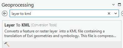
Figure 25.30 Searching for the Layer to KML tool
The layer is the random point feature class. Name the .kmz file appropriately and then Run the tool (Figure 25.31).
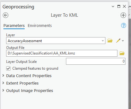
Figure 25.31 The Layer to KML tool
Like all geoprocessing tools, when the tool has finished, a completed message appears at the bottom of the tool (Figure 25.32). However, there is no new layer in Contents because this is not a file for use in ArcGIS but in Google Earth.

Figure 25.32 The Layer to KML tool processing status
The file is located in the folder for your project—not the geodatabase, just the project folder (Figure 25.33).
![]()
Figure 25.33 A KML File located in Windows Explorer
To open Google Earth, double-click on the file name, in this case, AA_KML. Google Earth will zoom directly to the location of the points, and the file will be listed in Temporary Places (Figure 25.34).
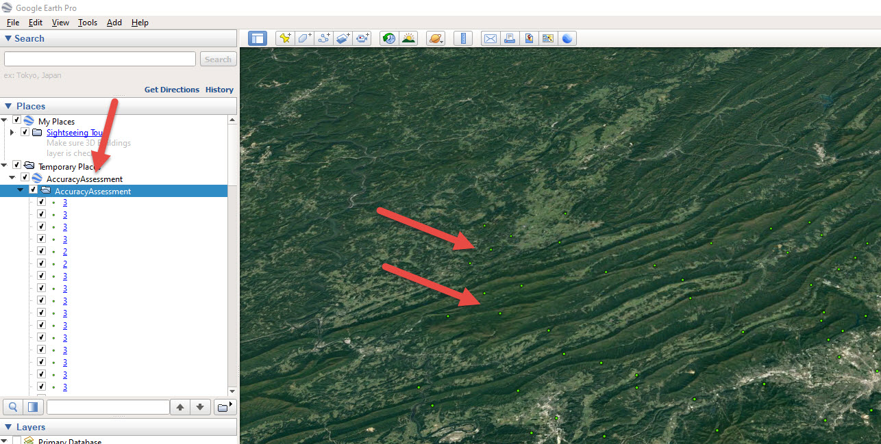
Figure 25.34 A KML file added to Google Earth
Using the historical image slider bar tool, locate the Google Earth image date that is closest to your Landsat date (Figure 25.35). To zoom into each point, double-click it under Temporary Places>Accuracy Assessment. As outlined above, you can manually add the value to the attribute table of the random point feature class in ArcGIS® Pro.
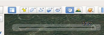
Figure 25.35 The Google Earth historical image toolbar
This concludes the chapter on accuracy assessment and the demonstration of remote sensing using ArcGIS® Pro.
As noted frequently, within each chapter, this book serves as a guide to using ArcGIS® Pro only; it does not provide sufficient information on making choices in remote sensing analysis specific to any individual project.
Endnote