24 Chapter 24: Conducting a Supervised Classification of a Landsat 9 Image

Introduction

Training samples have been created (Chapter 22) and evaluated (Chapter 23). In this final chapter on supervised classification, we provide details on completing a signature file and conducting the supervised classification. We introduce three alternative procedures to conduct this classification (please note that there are many other techniques and algorithms for conducting a supervised classification).

Objectives

The objectives of this chapter are to:

Generate supervised signatures using training samples.

Perform a supervised classification on a Landsat 8 image using the maximum likelihood geoprocessing tool.

Perform a supervised classification using the Classify Raster geoprocessing tool.

Perform a supervised classification using the Image Classification Wizard.

This chapter uses the 6-band subsetted composite Landsat 9 image. We will be using the same informational classes used in Chapters 21 – 23, so, as a reminder, the classes are:

Supervised Classification using Maximum Likelihood

We recommend that you open a new map project for this process. Add the 6-band subsetted composite image (created in Chapter 15) and the training sample shapefile created in Chapter 23, the final one created after evaluating spectral signatures. Do not use the shapefile with one training sample for each information class. Set the image to a natural color symbology and the training sample shapefile to unique values for the informational class color symbology noted above (Figure 24.1). Do not forget to set the workspaces.

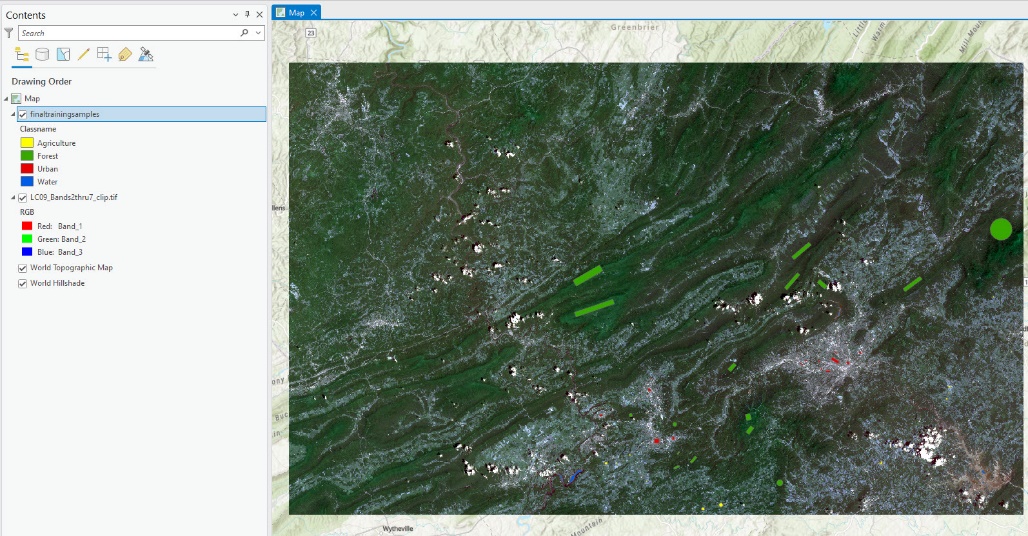
Figure 24.1 Composite image with training samples

Creating a signature file

We also need a signature file, a file with the spectral signatures for each informational class, to use the maximum likelihood tool.

Go to the Analysis tab on the Ribbon and select Tools. Search for Create Signatures. Figure 24.2.

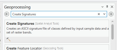
Figure 24.2 Searching for the Create Signatures tool

Open the tool (Figure 24.3).

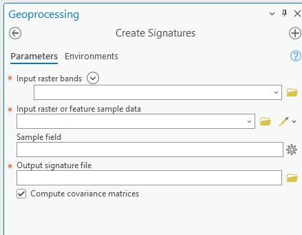
Figure 24.3 The Create Signatures tool

Input raster bands is the subsetted composite 6-band image. The Input raster or feature sample data is the training samples shapefile. Sample field should be classvalue. For the output signature file, name it, and navigate to and save it in the project file folder. (Processing note—when creating the signature file, the tool fails to run the first time; use the default folder location. When ArcGIS^® Pro software was added, it automatically created a default workspace and geodatabase. Sometimes, when a tool fails to run, try to let it save in these default locations. For this particular tool, it solves the failure problem).

Once all tool parameters are entered (Figure 24.4), select Run.

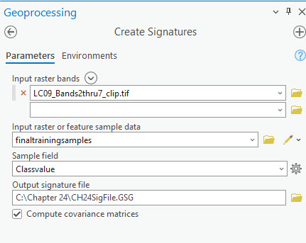
Figure 24.4 The Create Signatures tool

If successful, a Completed successfully message displays (Figure 24.5).

Figure 24.5 Completed Successfully message

But a new layer does not show in Contents (Figure 24.6).

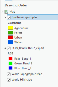
Figure 24.6 Contents without the signature file

However, the new file will be listed in the appropriate folder location on the computer (Figure 24.7). You do not need to add this file to Contents.

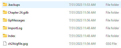
Figure 24.7 The signature file (.gsg) in Windows Explorer

Geoprocessing Tools – Conducting a Maximum Likelihood Classification

Go to the Analysis tab, open Tools, and search for Maximum Likelihood Classification (Figure 24.8).

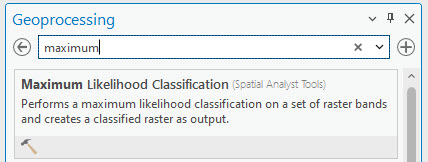
Figure 24.8 Searching for the Maximum Likelihood Classification tool

Open the Maximum Likelihood Classification tool (Figure 24.9).

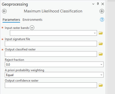
Figure 24.9 The Maximum Likelihood Classification tool

For the Input raster bands, select the 6-band composite image. The input signature file is the one we created above (.gsg file extension). If you cannot navigate to the .gsg file from the file folder within the tool, you can add it from the Windows environment. Open the File Explorer in Windows, navigate to the folder where the file is located and open it to view the list of files. Place the window showing the file side by side with ArcGIS^® Pro, and drag the .gsg file into the field. (Yes! ArcGIS^® Pro allows you to drag files into the program.)

Rename the Output classified raster. Leave Reject fraction at 0.0 because we want all cells to be classified. Leave A priori probability weighting at Equal. Under the Environments tab, do not change any settings. These settings can be changed depending on the needs of the final project but are optional here. The final inputs should look like Figure 24.10.

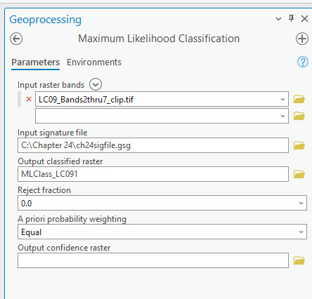
Figure 24.10 The Maximum Likelihood Classification tool

Select Run. Completed successfully displays when the tool finishes.

There is now a new layer in Contents and a new image displayed in the map viewer (Figure 24.11).

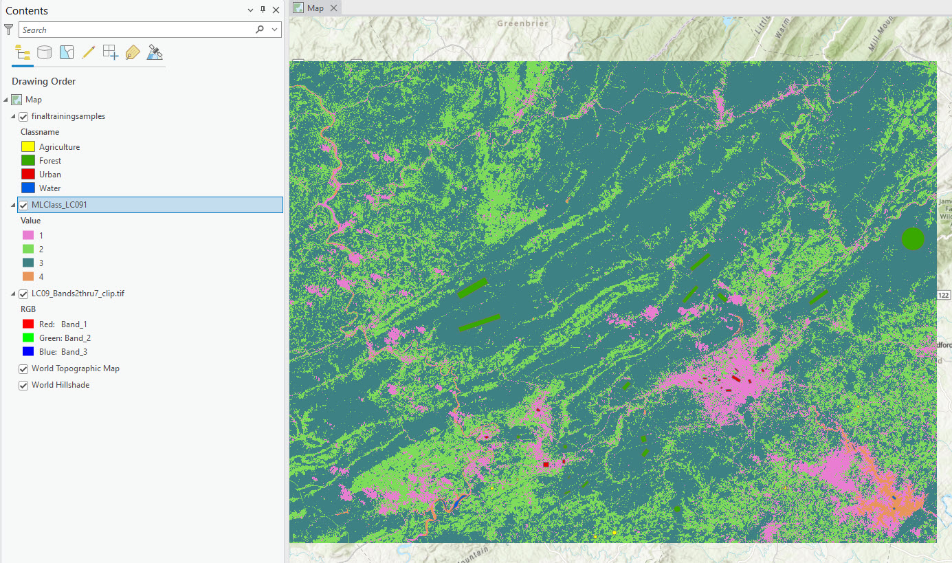
Figure 24.11 Map display showing results of the ML image

As usual, the symbology is randomly selected, so correct by changing Water to blue, Urban to red, Forest to green, and Agriculture to yellow (Figure 24.12).

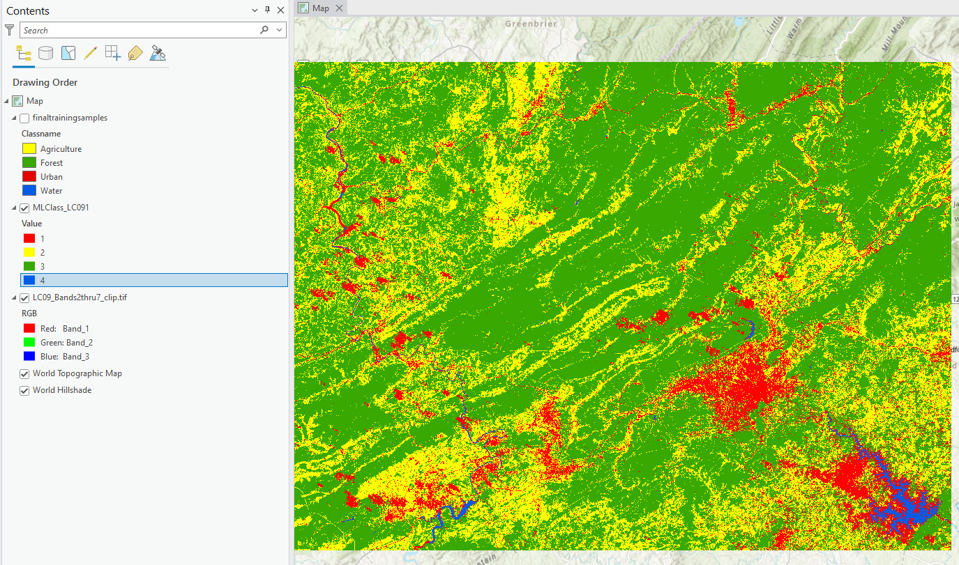
Figure 24.12 Corrected symbology

Calculating the Percent of Total Area for Each Informational Class

Calculate the number of hectares and the percent of total land cover for each informational class (Figure 24.13) as demonstrated in Chapter 21 – Unsupervised Classification. Do you remember how to do this?

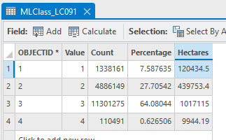
Figure 24.13 Calculation of area for each informational class

How accurate was your classification using the Maximum Likelihood Classification method? We will assess that in Chapter 25: Accuracy Assessment. We will use this maximum likelihood image and the percentages from the attribute table in that chapter. However, before proceeding to that chapter, we will demonstrate two additional classification processes in ArcGIS^® Pro.

Geoprocessing Tools–the Classify Raster Tool

Geoprocessing tools provide additional options for classification. Under the Analysis tab, open Tools and search for “Classify Raster” (Figure 24.14).

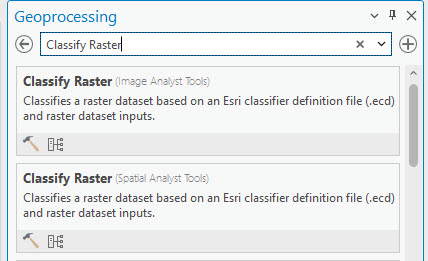
Figure 24.14 Searching for the classify raster tool

Open the Classify Raster (Spatial Analyst Tools). As you can see from this tool, we need to specify an additional file—a definition file¹ (Figure 24.15).

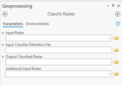
Figure 24.15 The classify raster tool

So, return to the search and find the Train Maximum Likelihood Classifier (Image Analyst Tools) (Figure 24.16).

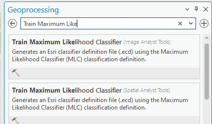
Figure 24.16 Searching for the Train Maximum Likelihood Classifier tool

Open the Train Maximum Likelihood Classifier tool and enter the parameters as shown in Figure 24.17. Dimension Value Field and Additional Input Raster are optional; leave these empty. Do not change anything under Segment Attributes.

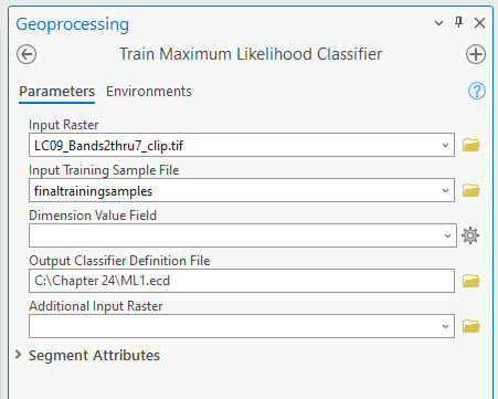
Figure 24.17 The Train Maximum Likelihood Classifier tool

Select Run, and once complete, a Completed successfully message displays. There will not be a new layer in Contents.

Now that we have a definition file, we can use Classify Raster. The inputs for this tool are shown in Figure 24.18. Once entered, select Run.

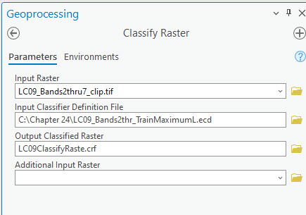
Figure 24.18 The classify raster tool

A Completed Successfully message will display, and a new layer appears in Contents with a new image in the Map. With this method, because the training sample shapefile was used to create the definition file (.ecd), the symbology carried over to the new image (Figure 24.19).

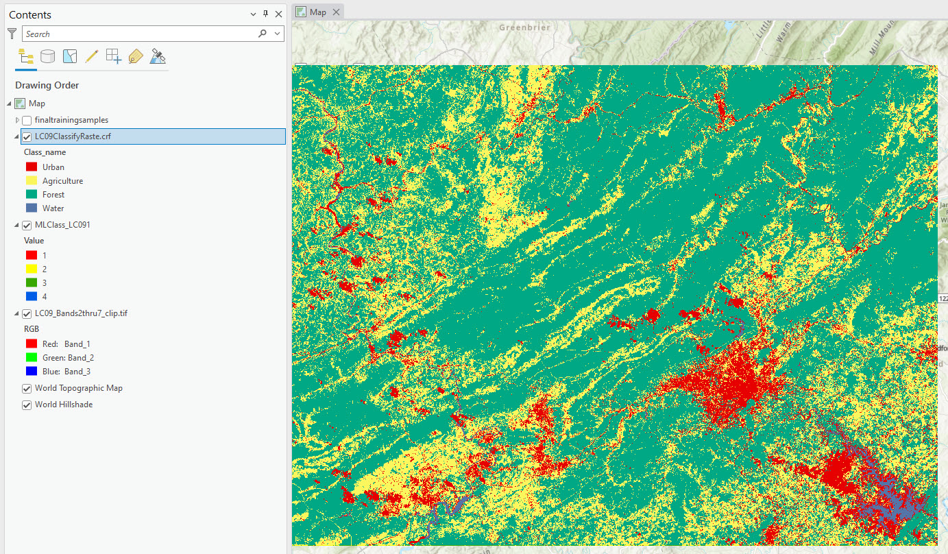
Figure 24.19 The classify raster image in the map display

However, this method does not provide a cell count (Figure 24.20), so calculating the number of hectares or the percent of informational classes requires additional geoprocessing steps. We will demonstrate this process in the next section when we demonstrate the Classification Wizard ².

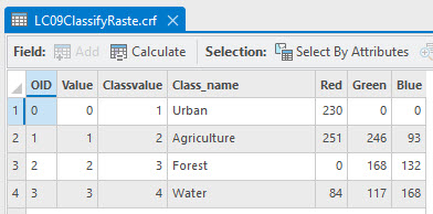
Figure 24.20 Attribute table from the new file

Be sure to save your project before proceeding.

Image Classification Wizard

We briefly reviewed the Image Classification Wizard in Chapter 21: Unsupervised Classification and Chapter 22: Introduction to Supervised Classification.

Go to the Imagery tab and select Classification Wizard (Figure 23.21). If the button is not enabled, be sure you have selected the 6-band subsetted composite image in Contents.

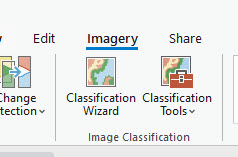
Figure 24.21 The Classification Wizard

In the Wizard, under Classification Method, choose Supervised. Then under Classification Type, choose Pixel-based. Under Classification Schema, we have four options. Remember from Chapter 22 that we already created a classification schema based on the NLCD 2011 schema, so browse to the location where that training sample schema was saved (.ecs) and add it.

Under Optional, add the training samples shapefile. Once your tool mirrors Figure 24.22, select Next at the bottom.

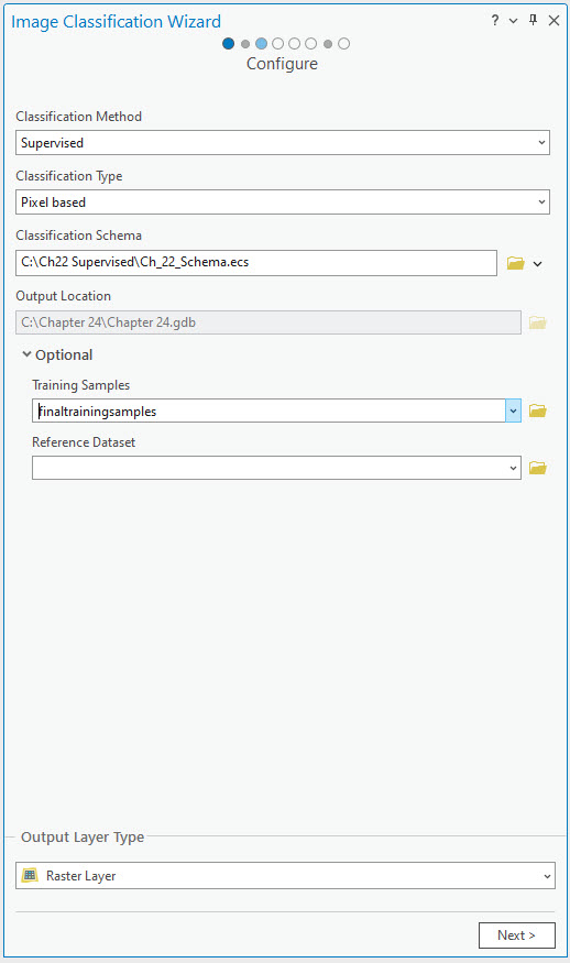
Figure 24.22 The Classification Wizard

Had we not already created the training samples, they can be created here. But as you can see in Figure 24.23, our shapefile populated the training samples area.

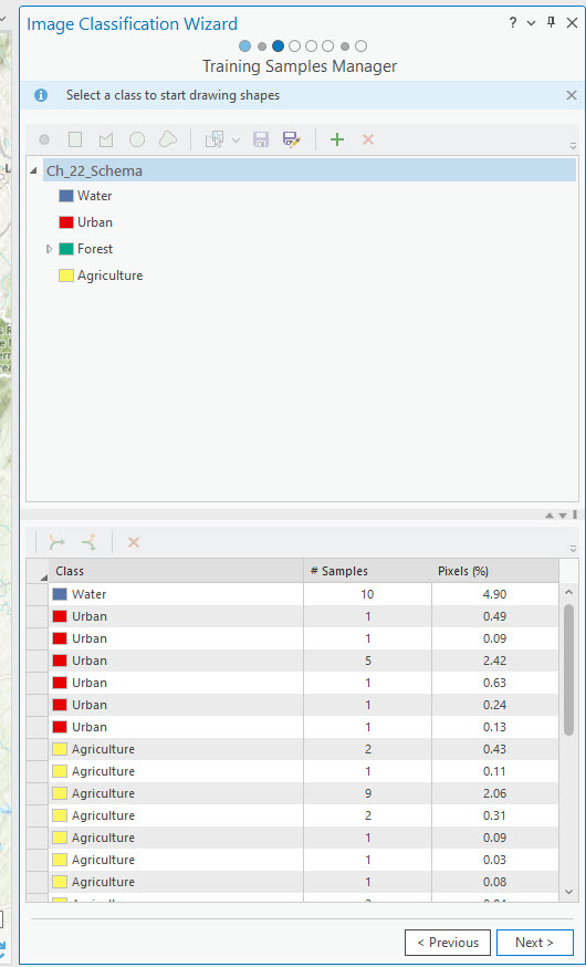
Figure 24.23 The Classification Wizard

Select Next again. Maximum Likelihood is one of several options within the Image Classification Wizard (Figure 24.24), we already demonstrated that option above, so will use a different option here.

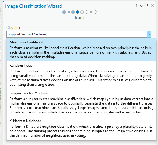
Figure 24.24 Classification Wizard options

Select the Classifier Support Vector Machine. See the description of this classification method in Figure 24.24. Then click Run. This processing might take a bit longer than the prior classification methods.

Once the processing is done, a Completed successfully message displays, a new layer is in Contents, and a new image is in the map viewer (Figure 24.25). The new image has the appropriate symbology because we again used the classification schema (.ecs). Caution, the image is only available in this project. So, if completing an accuracy assessment with this image, the accuracy assessment must be accomplished within this project.

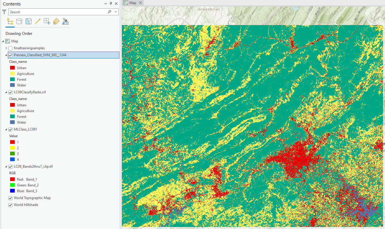
Figure 24.25 Support Vector Machine classification result

You can export it into a permanent file by right-clicking on the file name and choosing Data > Export Raster (Figure 24.26). We will not demonstrate that step here.

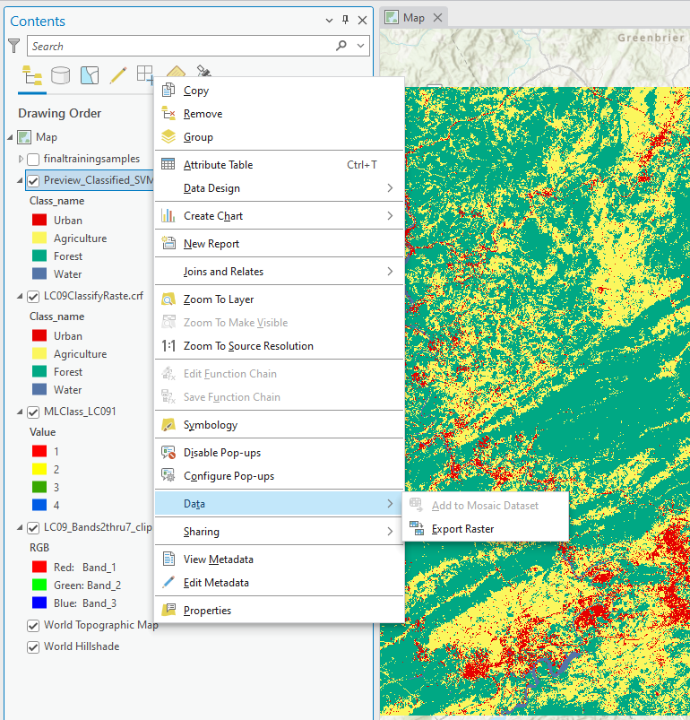
Figure 24.26 Exporting the data to a new permanent file

Please note that while this image file does have an attribute table (Figure 24.27), it also does not have a count of the number of cells associated with each informational class, as happened with the Classify Raster method discussed in the prior section.

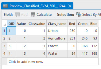
Figure 24.27 An attribute table with the SVM classified image

These results show that the number of hectares and percentage of land use cannot be calculated based on the cell count without additional geoprocessing tools. We will demonstrate this in the next step.

Go to Analysis, Tools and search for “Cell Statistics”. Open the tool.

The Input raster is the Preview_Classified_SVM_500_1244 generated from the Image Classification Wizard. Name the Output Raster and choose Sum from the list of Overlay Statistics (Figure 24.28). Then select Run at the bottom. Running this tool does take a few minutes; we are dealing with tens of thousands of pixels.

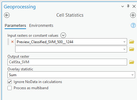
Figure 24.28 Cell statistics tool populated

A new file is in Contents, and a new image is in the map viewer (Figure 24.29).

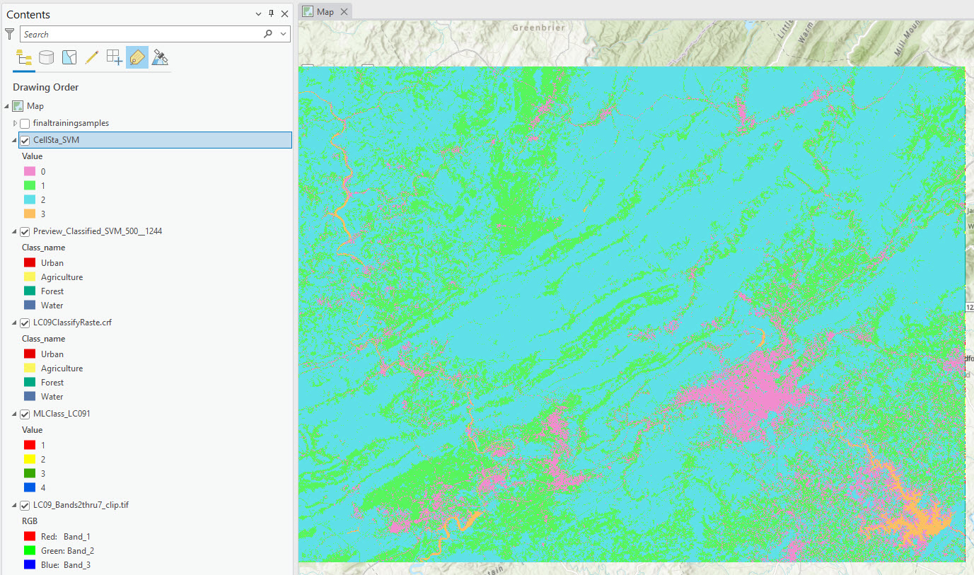
Figure 24.29 New SVM classified image

Open the Attribute Table for this new layer, and a cell count by value is now present (Figure 24.30).

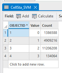
Figure 24.30 Attribute Table from New SVM Classified Image

Although the classification scheme numbering (value field) has changed, the relationship of the value field to the informational class can easily be verified and corrected by using your other classified images as a reference. Now, add fields into this attribute table for Classname, Hectares, and Percentage, and calculate the values. (Figure 24.31).

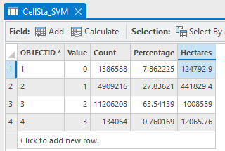
Figure 24.31 Attribute table with new fields calculated

Again, we note that only four classification algorithms for supervised classification are available with the Wizard. For more information on the Image Classification Wizard, refer to: https://pro.arcgis.com/en/pro-app/help/analysis/image-analyst/the-image-classification-wizard.htm.

This concludes the chapter on supervised classification. We will use the files created using the classified images Maximum Likelihood and Support Vector Machine, along with the image created in Chapter 21 Unsupervised Classification, in the final chapter Chapter 25 Accuracy Assessment.