16 Chapter 16: Band Combinations for Landsat 9 Imagery
Introduction
This chapter discusses band combinations and how to use them within ArcGIS® Pro. We begin with a brief review of Landsat 9 spectral channels and a discussion on band combinations, spectral values for features on the surface of the Earth, and how different features can be identified using specific bands.
Each of the 11 Landsat 9 bands covers a different region of the electromagnetic spectrum. By combining three or more bands, images (outside of the visible spectrum) can be associated with red, green, and blue (RGB) colors. Remember from prior chapters discussing Landsat 9 imagery that each spectral channel (designated as a band for satellite imagery) is defined by its distinctive region of the electromagnetic spectrum. Each band is specifically tailored to help distinguish and observe specific features on the Earth’s surface. See Figure 16.1 for Landsat 9 band uses. Notes at the end of this chapter provide additional details on the usefulness of individual bands and band combinations for identifying specific surface features.
Different features on the surface of the Earth respond to various wavelengths of the electromagnetic spectrum; features absorb, reflect, and re-emit the radiation in different ways. Using various band combinations to display the scene in color allows these dissimilar features to be more easily detected and identified. This process does take some experience, and users must become familiar with the scene to identify, for example, urban areas, forests, agriculture, and water bodies. Familiarity with the satellite platform (Landsat or Sentinel, for example) is vital for analyses such as unsupervised classification, supervised classification, and different indices such as NDVI, covered in Chapter 19: Spectral Enhancement of Landsat 9 Imagery. Several types of analyses are covered in subsequent chapters.
Using data outside the visible spectrum
Examine the tables at the end of this chapter. These tables provide several examples of how data outside the visible spectrum can be used to observe features more effectively on the Earth’s surface. For example, the near-infrared (NIR) wavelengths are very useful for water bodies, as clear, calm water absorbs NIR wavelengths. Thus, water bodies appear very dark, almost black, on a color infrared image. Additionally, healthy, vigorous vegetation is more readily identified using the NIR bands, much more so than the green band. Figure 16.1 provides general information regarding the potential applications of various wavelengths of Landsat 9.
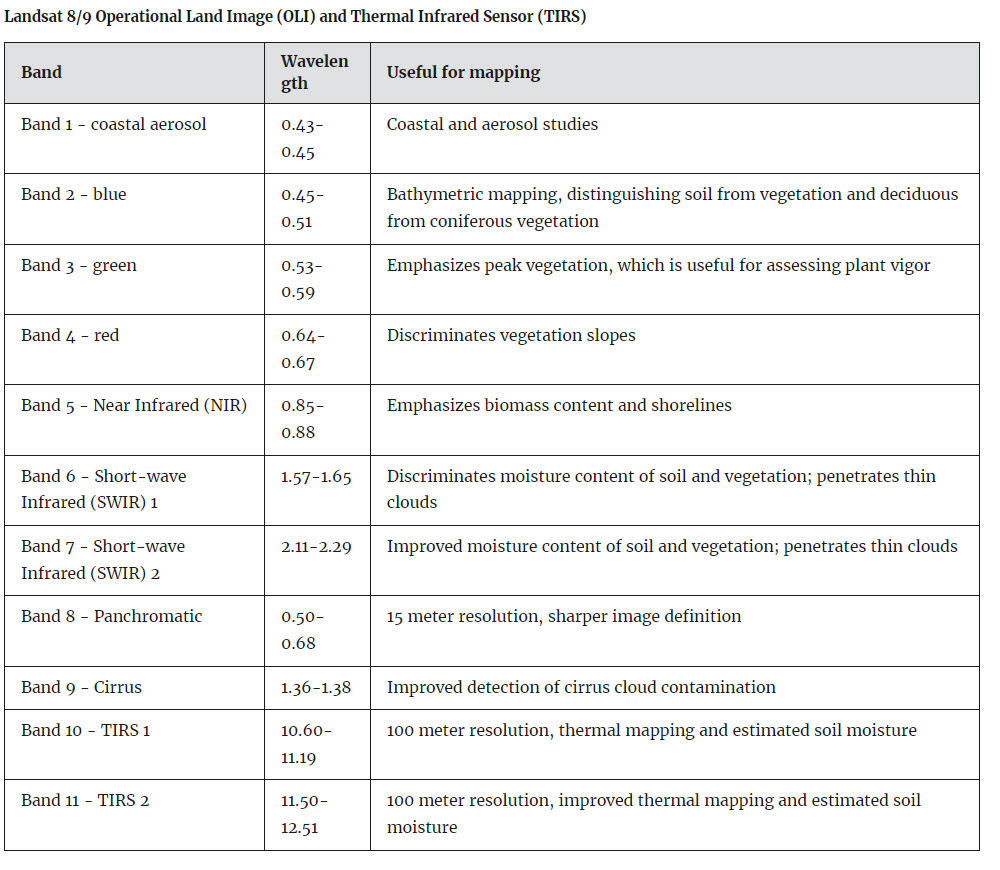
Figure 16.1 Landsat 8/9 bands and associated mapping applications. Source: USGS. https://www.usgs.gov/faqs/what-are-best-landsat-spectral-bands-use-my-research
An in-depth discussion of the spectral properties of individual features on the Earth’s surface is beyond the scope of this book. Additional information about this topic can be acquired from various online resources, including:
- https://www.usgs.gov/media/images/common-landsat-band-combinations
- https://earthobservatory.nasa.gov/Features/FalseColor/page6.php
- http://www.mngeo.state.mn.us/chouse/airphoto/cir.html
- https://web.pdx.edu/~nauna/resources/10_BandCombinations.htm
- https://publiclab.org/wiki/near-infrared-imaging
- https://gisgeography.com/landsat-8-bands-combinations/
Recall from Chapter 10 that when downloading scenes collected from a specific satellite platform, it is important to note that each band conveys information. Unfortunately, the band numbers’ spectral properties are often inconsistent between satellite platforms (even if the band numbers are the same). For example, the spectral properties of a Band 5 image collected by Landsat 4 will not match the spectral properties of a Band 5 image collected by Landsat 9. We have attempted to consolidate much of the information associated with the bands of the Landsat family (Landsat 1-9) in the “Additional Notes” section at the end of this chapter. For more information associated with the Landsat program, please consult information provided by the USGS: https://www.usgs.gov/faqs/what-are-band-designations-landsat-satellites .
Creating Different Band Combinations
This section will provide step-by-step instructions to change and explore band combinations of Landsat 9 imagery using ArcGIS® Pro.
Open ArcGIS® Pro. This section will use the subsetted composite image created from bands 2-7, Chapter 15: Subsetting a Composite Landsat 9 Image (Figure 16.2).
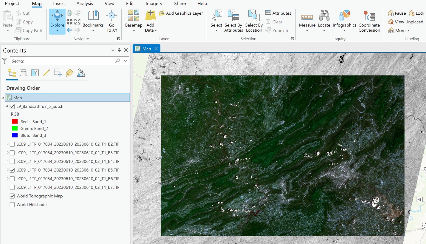
Figure 16.2. Subset of the original image with a grey-scale image in the background for reference
There are several ways to assign color and change the combination of bands for a composite image. We will start with two default options.
Short Cut Button for Band Combinations
Select the composite image in Contents and click the Raster Layer tab. Under this tab is a button called Band Combination (Figure 16.3).
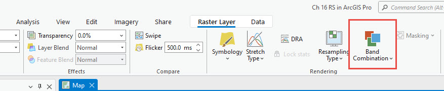
Figure 16.3. The Band Combination button
Select Band Combination. Three options are in the drop-down list—Natural Color, Color Infrared, and Custom (Figure 16.4). Each option will be discussed, but more so as a cautionary note when using this shortcut. This will become clear as we proceed.
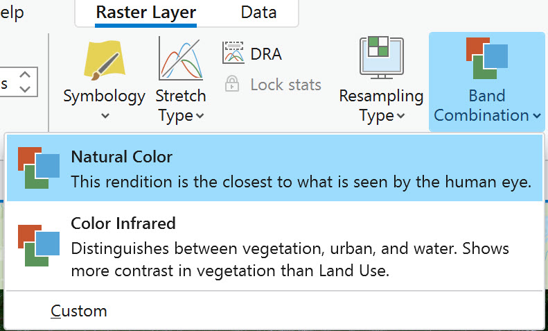
Figure 16.4 The Natural Color option
Point to Natural Color to view a pop-up explanation of its meaning (Figure 16.5).
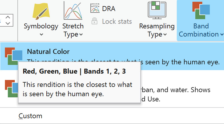
Figure 16.5 The Natural Color pop-out box
Natural color uses the wavelengths of the electromagnetic spectrum in the visible range—red, green, and blue (what ArcGIS® Pro calls Bands 1, 2, 3) to display the image. Figure 16.1 depicts Band 2 as Blue (not Red), Band 3 as Green (not Blue), and Band 4 as Red. ArcGIS® Pro defaults to Red for Band 1, Green for Band 2, and Blue for Band 3. Blue is a shorter wavelength than Red, so the Blue band actually comes first in the visible range of the electromagnetic spectrum and the labeling for satellite bands. ArcGIS® Pro numbers the bands in numerical order; the band number is unrelated to the spectral properties of the bands.
Point to the Color Infrared option (Figure 16.6).
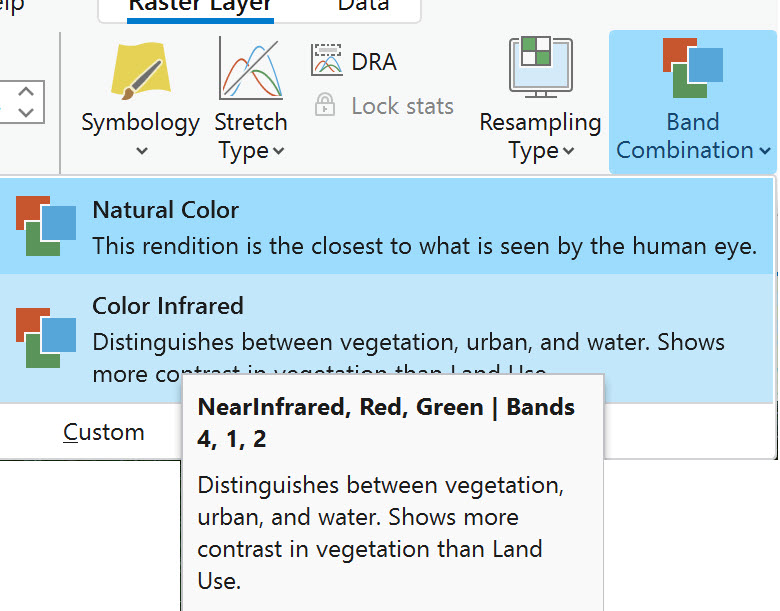
Figure 16.6 The Color Infrared pop-out box
Color infrared uses wavelengths from the green and red visible wavelengths and the wavelengths from the next region of the electromagnetic spectrum—near-infrared. But again, the band designations in ArcGIS® Pro do not correspond to the band sequence of Landsat 9, as Band 5 should be associated with the near-infrared band.
The third option under band combinations is Custom. Using this option, users can set a specific band combination to use regularly. When using Landsat 9 Natural Color regularly (and using all 11 bands), set the Custom parameters to Band_4 for red, Band_3 for green, and Band_2 for blue to generate a true color image. However, keep in mind that our composite image only includes seven of the eleven bands. Name your custom display Landsat 9 Natural Color (Figure 16.7). Be careful when setting these values. Therefore, the band combination a true color image for this image is 3-2-1.
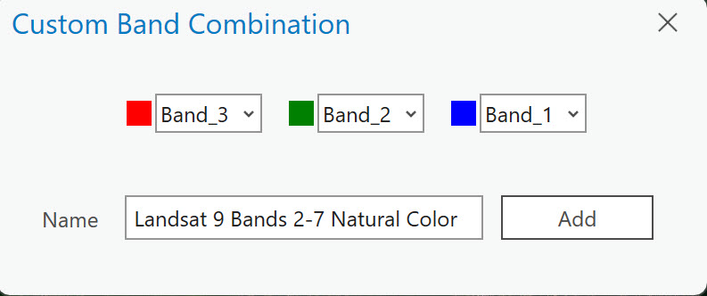
Figure 16.7 The Custom Band Combination option
Click Add, and we have a natural color, 321 Band Combination Landsat 9 image. The image in the display window (Figure 16.8) does now look more like features seen on the Earth. This is how natural color (or true color) should appear.
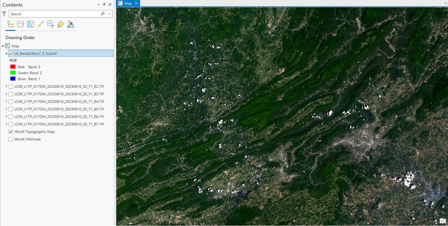
Figure 16.8 Displaying a Landsat 9 image in true color
Use the Custom setting again, but use the band combinations for Landsat 9 Color Infrared (hint: refer to the USGS’s Common Landsat Band Combinations webpage (https://www.usgs.gov/media/images/common-landsat-band-combinations).
After creating a Color Infrared image, your display window should appear similar to Figure 16.9. Does your image look like the one below? When using an 11-band composite image, the Landsat 9 bands for Color Infrared are 5-4-3 (Band 5 = red, Band 4 = green, and Band 3 = blue). However, since we are using a composite image using bands 2-7 (our composite image is missing band 1), the Color Infrared image must utilize the 4-3-2 band sequence (Band 4 = red, Band 3 = green, and Band 2 = blue).
 Figure 16.9 A Color Infrared image.
Landsat 9’s Band 5 (in this case labeled by ArcGIS® Pro as Band 4) is the near-infrared band. Normally, we cannot see data from this segment of the electromagnetic spectrum, but we have arranged the NIR band so that ArcGIS® Pro will display it in red. Using this band combination, vegetation appears bright red. Healthy or more vigorous vegetation is highly reflective in the near-infrared band. The healthiest vegetation, or mature vegetation at its peak within this scene, will show as deep/dark red. That does not mean the land cover associated with pink hues (less red saturation) is unhealthy vegetation. It is possible, for example, that this vegetation could be less dense or less mature. This exemplifies the importance of in-situ verification.
There is a tremendous difference between the two images: Natural/True color and Color Infrared. We will discuss the differences in more detail a bit later. But first, we will explore another option for changing and visualizing different band combinations of a composite image.
Band Combinations using Symbology
Open Symbology for the image. Recall that you can access Symbology from the Raster Layer tab on the ribbon or by right-clicking the layer in Contents.
With Symbology, we can create any band combination we want using the drop-downs for the bands next to each color in the Primary Symbology. Again, it is vital to remember which bands were used when creating the composite image. If all eleven Landsat 9 bands, beginning with Band 1 and adding them in order, were not used, the band numbers would be different in ArcGIS® Pro than what the actual Landsat designations are. This information must be retained when doing analyses. And remember, we are assigning different wavelengths of the electromagnetic spectrum to colors we can see with the naked eye. Humans are unable to see the NIR and other nonvisible wavelengths. But with the software’s help, we can display them with color and are therefore able to visualize them. Keep in mind that, through remote sensing, we are actually visualizing how these different bands are either absorbed or reflected when they interact with features on the Earth’s surface.
Once Symbology opens, change band numbers to the appropriate colors (Figure 16.10). Right now, for our image, the combination is 4-3-2.
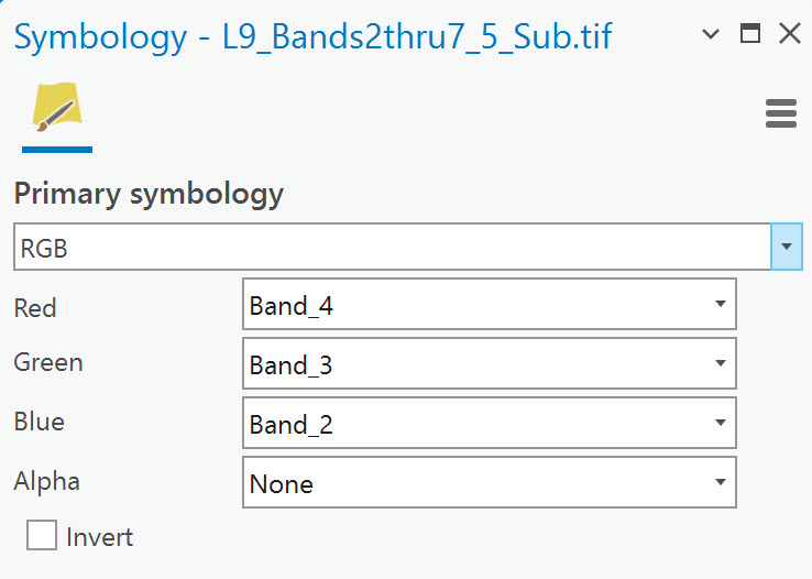
Figure 16.10 Changing band symbology
Using the drop-down arrow at the end of each color’s field, change Red to Band_3, Green to Band_2, and Blue to Band_1. This is the natural color combination for this image subset (compare this to the natural color combination for an 11 band image here (https://www.usgs.gov/media/images/common-landsat-band-combinations). Your image display should look similar to Figure 16.11.
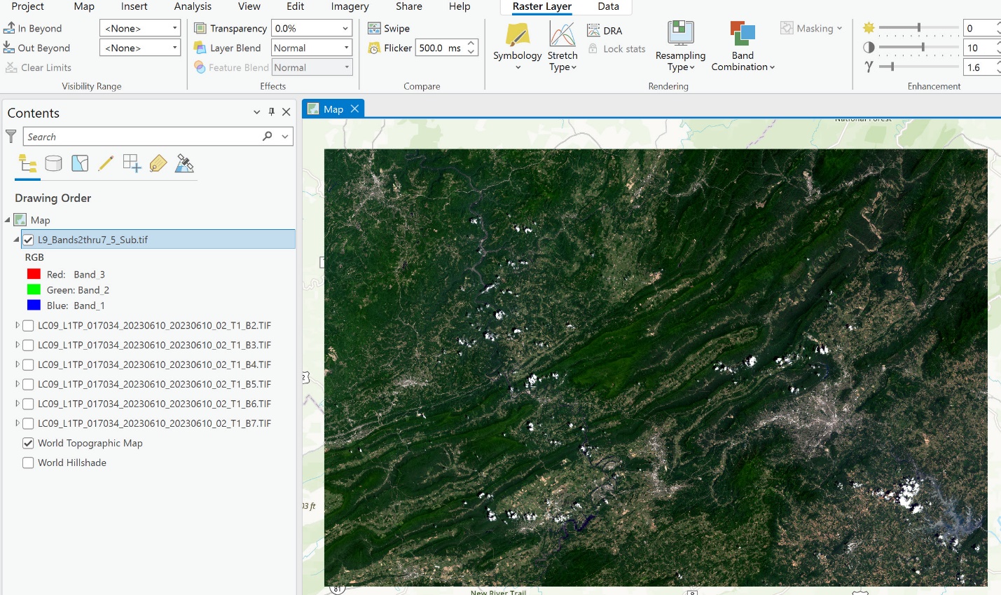
Figure 16.11 Displaying a Landsat 9 scene
Now change the image to Color Infrared. Your displayed image should look similar to Figure 16.12.
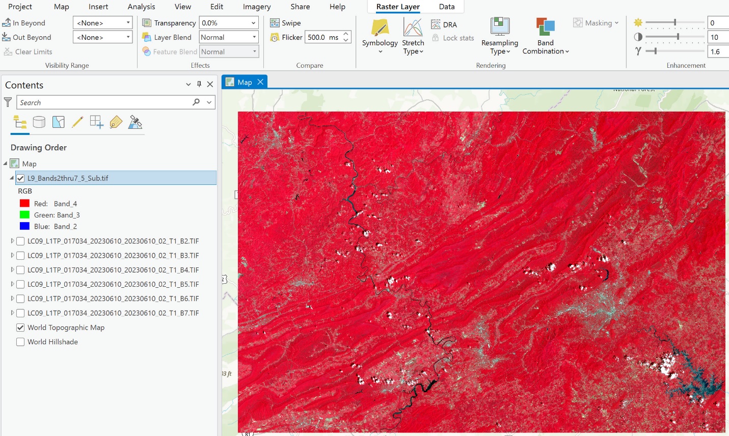
Figure 16.12 Displaying a Landsat 9 image in color infrared
Let’s compare the true color and near infrared images. The following two figures (16.13 and 16.14) are the Natural Color compared to the Color Infrared. Can you identify some specific differences?
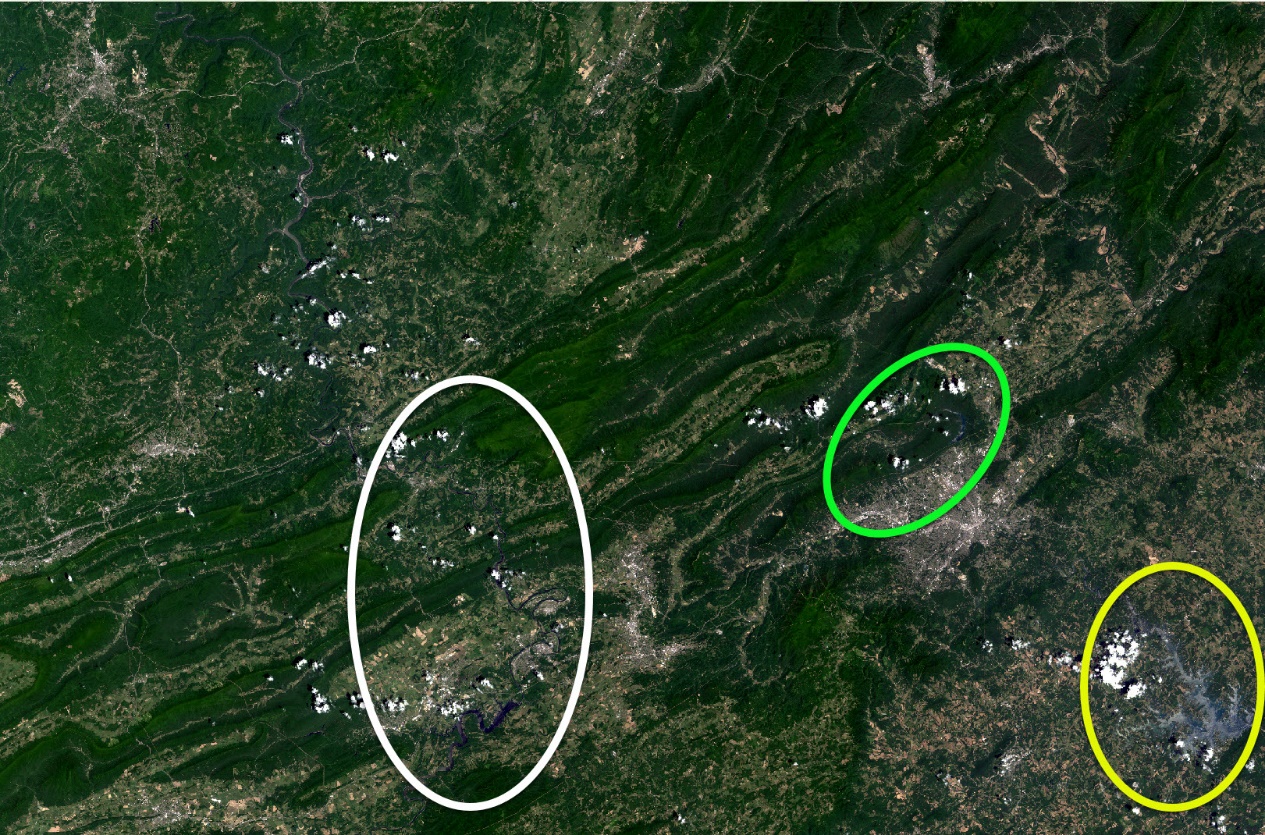
Figure 16.13 True color Landsat scene with highlighted regions for comparison
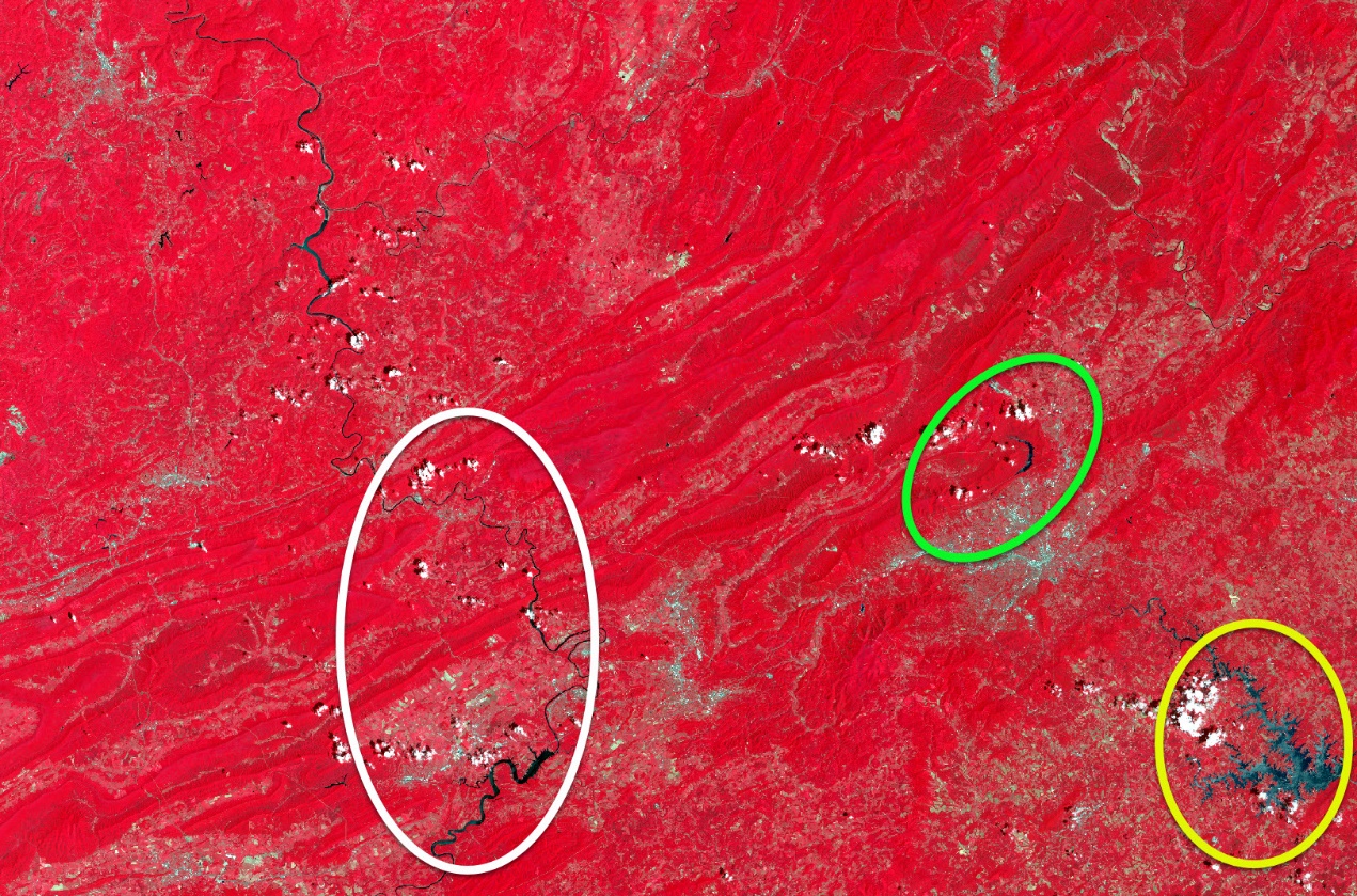
Figure 16.14. False color Landsat scene with highlighted regions for comparison
Within the three ovals in the two images above are water bodies. Inside the white oval is the New River. The New River is fairly evident in the Natural Color image, especially the southern wider portion of the river. In the Color Infrared, the river’s entire course is quite apparent. The lime green circle in the north is Carvin’s Cove, a drinking water reservoir for the City of Roanoke. Carvin’s Cove is barely visible in the Natural Color image but is very prominent in the Color Infrared image. Finally, Smith Mountain Lake, located in the southeast section of the image, is situated in the yellow circle. Now that we have pointed it out, you can make out the lake in the Natural Color image, but it is clearly evident in the Color Infrared image. Additionally, note that the lake is not all dark. Smith Mountain Lake is a reservoir, and north of the dam, the river flowing into the lake is heavily laden with sediment, which appears as a bright light blue in the image.
How do these two image combinations display vegetation? Green in the true color image is associated with vegetation. This is a summer image in Virginia (June 10, 2023), and within this region are extensive forests, including both a National Forest and a State Forest. Red in the second image shows the vegetative cover much more prominently. Virginia is a heavily vegetated state with both forests and agriculture.
Now zoom in. The agriculture fields appear as lighter shades of green in the True Color image and as various shades of pink in the Color Infrared image (Figure 16.15).
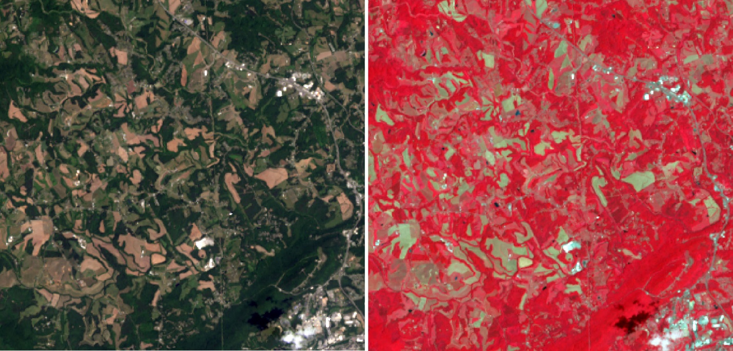
Figure 16.15 Comparing true color and a false color NIR image
Let’s try another area of the scene– the city of Roanoke. Roanoke is the largest urban area in southwest Virginia and within this Landsat scene. What do you find in urban areas (hint: long linear features like roads, things with definite angles like buildings, perhaps an airport)? Can you find the city?
Zoom into the City of Roanoke (Figure 16.16). Can you identify any features within the city, such as roads, the airport, and some golf courses?
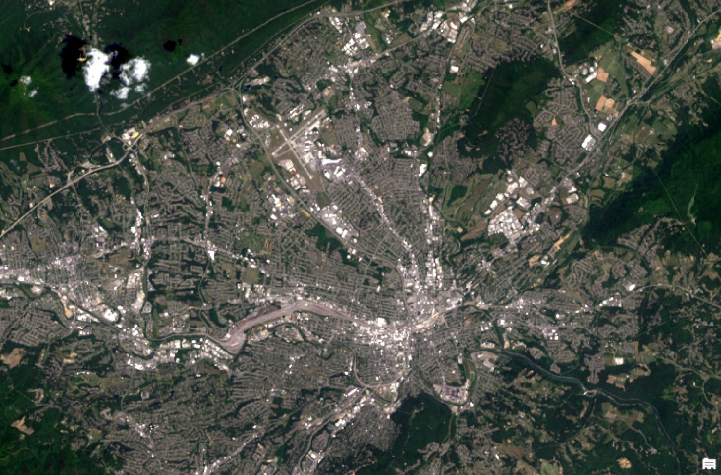
Figure 16.16 Landsat 9 image from the City of Roanoke
Remain zoomed into Roanoke and now explore the city using a Color Infrared display (Figure 16.17). Roanoke looks a lot different. The Roanoke River runs through Roanoke southeast to Smith Mountain Lake. The river is barely visible in the Natural Color image (can you see it?). In the Color Infrared image, the river is visible in the southeast of Roanoke, but the river almost disappears within Roanoke.
Can you identify any golf courses? (Hint: healthy vegetation is bright red in a false color infrared image—what do you find in a golf course year-round?) What other features on a golf course might be visible with Landsat imagery? Can you identify the fairways and putting greens along the golf courses? What about sand traps? Would sand traps be displayed as bright red on a Color Infrared image?
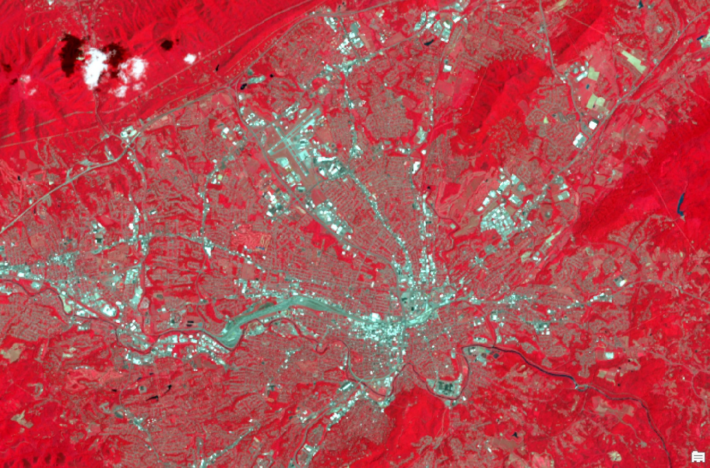
Figure 16.17. A false color NIR image of Roanoke
The images in Figure 16.18 show a portion of Roanoke using different band combinations: Natural Color (left), Color Infrared (middle), and a new band combination (more information about this image later!). You can see that there are distinct differences between these three images—they each highlight different features on the Earth.
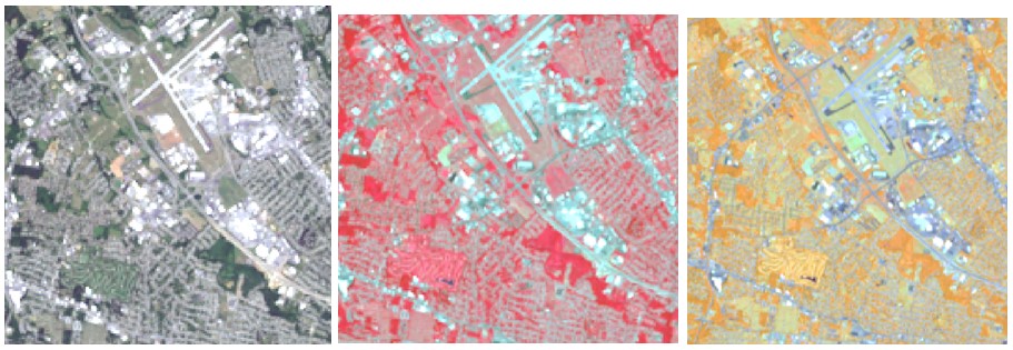
Figure 16.18. Comparing Roanoke using various band combinations from Landsat 9
The third image (on the right and in Figure 16.19) uses a band combination of 5-6–8. This is impossible given that we do not have band 8 in our composite image, but using the combination 4-5-3 will make one similar. All the bands associated with the 5-6-8 image are outside the visible spectrum. But the river channel is now a distinct line meandering on the south side and through the city.
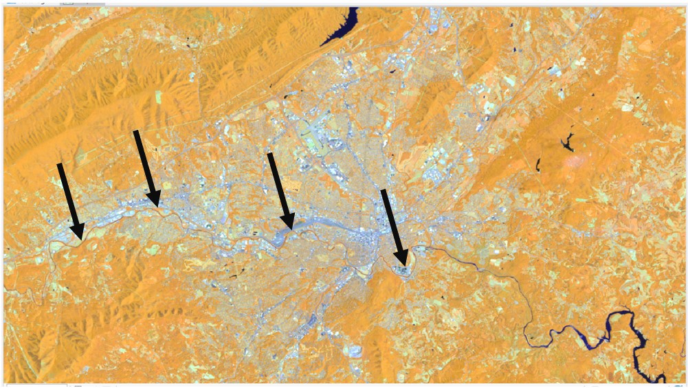
Figure 16.19. Landsat 9 image showing a river channel
Why do the different bands placed within those specific channels make a difference? See the Landsat 9 Table in Figure 16.1 and additional notes at the end of this chapter.
What other features can you identify with this band combination that you could not discern from the natural color combination? The same band can be used multiple times. Figure 16.20 is a 7-5-7 spectral band combination the image (ArcGIS® Pro numbering 6-4-6 for our composite).

Figure 16.20 A Landsat 9 color composite
Again, note that the same band can be displayed more than once—in the example above, band 6 (Landsat band 7) was assigned to two different colors in ArcGIS® Pro. This again changes the display in the map document window. Does this band combination facilitate seeing anything more distinctly in the forested mountains? No, Band 4 (near infrared) is the most effective band for observing differences in vegetation vigor, and Band 4 is not used in this combination. But the water bodies are even more prominent, and, in this image, we can even see some smaller water bodies and another river in the northeast, barely visible in the 5-4-3 Color Infrared combination (shown in various locations within the black ovals in Figure 16.21).
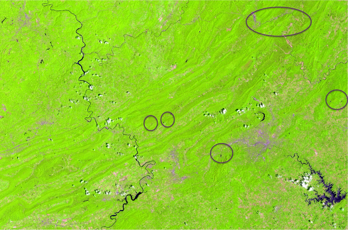
Figure 16.21 A Landsat 9 color composite
Go ahead and explore different band combinations. Follow the tables and charts at the end of this chapter. Try different combinations for the whole scene and other localized regions by zooming in.
Many aerial images from airplanes, drones, and other platforms within the Earth’s atmosphere, are acquired in 4 bands—the three visible bands (RGB) and the near-infrared. The USDA NAIP (National Agriculture Imagery Program) imagery is often acquired with four bands because the purpose of that program is to evaluate agricultural productivity, and these images are usually acquired during the growing season. 1 This 4-band imagery can be loaded into ArcGIS® Pro and displayed using the different band combinations, or it can be loaded with a GIS Server connection (see Chapter 4: Connecting to a Folder or an Online GIS Server). NAIP images are typically distributed as single, 4-band, composite images, not as separate image bands as Landsat imagery.
You are now ready to proceed to the next set of chapters, which discuss image enhancement techniques. The following pages of this chapter describe single-band sensitivities and specific band combinations.
ADDITIONAL NOTES
Single Band Sensitivities
LANDSAT Thematic Mapper (TM &ETM+)
0.45-0.52 μm BLUE (BAND 1)
•Shorter wavelengths most sensitive to atmospheric haze, so images in this region may lack tonal contrast
•Shorter wavelengths have greatest water penetration (longer wavelengths more absorbed); optimal for detection of submerged aquatic vegetation (SAV), pollution plumes, water turbidity, and sediment
•Detecting smoke plumes (shorter wavelengths more easily scattered by smaller particles
•Good for distinguishing clouds from snow and rock and soil surfaces from vegetated surfaces
0.52-0.6 μm GREEN (BAND 2)
•Sensitive to water turbidity differences, sediment, and pollution plumes
•Covers green reflectance peak from leaf surfaces, can be useful for discriminating broad vegetation classes
•Also useful for detection of SAV
•Also useful for penetration of water for detection of SAV, pollution plumes, turbidity, and sediment
0.63-0.69 μm RED (BAND 3)
•Sensitive in a strong chlorophyll absorption region, i.e., good for discriminating soil and vegetation
•Senses strong reflectance regions for most soils
•Effective for delineating soil cover
0.76-0.9 μm NEAR IR (BAND 4)
•Distinguishes vegetation varieties and vegetation vigor
•Water is a strong absorber of NIR, so this band is good for delineation of water bodies and distinguishing between dry and moist soils
1.55-1.75 μm MID OR SWIR (BAND 5)
•Sensitive to changes in leaf-tissue water content (turgidity)
•Sensitive to moisture variation in vegetation and soils; reflectance decreases as water content increases
•Useful for determining plant vigor and for distinguishing succulents vs. woody vegetation
•Especially sensitive to presence/absence of ferric iron or hematite in rocks (reflectance increases as ferric iron increases)
•Discriminates between snow and ice (light-toned) and clouds (dark-toned)
2.08-2.35 μm MID OR SWIR (BAND 7)
•Coincides with absorption band caused by hydrous minerals (clay mica, some oxides, and sulfates) making them appear darker; e.g., clay alteration zones associated with mineral deposits such as copper
•Lithologic mapping
•Like band 5, sensitive to moisture variation in vegetation and soils
10.4-12.5 μm LWIR, THERMAL (BAND 6)
•Sensor designed to measure radiant surface temps -100 degrees C to +150 degrees C; day or nighttime use
•Heat mapping applications: soil moisture, rock types, thermal water plumes, household heat conservation, urban heat generation, active military targeting, wildlife inventory, geothermal detection
Electromagnetic Spectrum and Band Coverage – Landsat 4, 5, 7, 8 and 9
Landsat 9 uses more bands relative to those of sensors used by the earlier Landsat satellites. In addition, Landsat 9’s divisions of the electromagnetic spectrum differ from those of TM and ETM+ sensors aboard Landsat 4, 5, and 7. See the following table for comparisons. When working with Landsat 9 imagery, be careful to use the appropriate bands when selecting band combinations.
|
Band Number |
Landsat 8 & 9: Operational Land Imagers (OLI) & Thermal Infrared Sensor (TIRS) |
Landsat 4 & 5: Thematic Mapper (TM) Landsat 7: Thematic Mapper Plus (ETM+) |
|
1 |
0.43 – 0.45 μm – coastal aerosol |
|
|
2 |
0.45 – 0.51 μm – blue |
|
|
3 |
0.53 – 0.59 μm – green |
0.52 – 0.61 μm – green |
|
4 |
0.64 – 0.67 μm – red |
0.63 – 0.69 μm – red |
|
5 |
0.85 – 0.88 μm – NIR |
0.76 – 0.90 μm – NIR |
|
6 |
1.57 – 1.65 μm – SWIR 1 |
1.55 – 1.75 μm – SWIR |
|
7 |
2.11 – 2.29 μm – SWIR 2 |
10.40 – 12.50 μm – thermal |
|
8 |
0.50 – 0.68 μm – Panchromatic |
2.08 – 2.35 μm – SWIR |
|
9 |
1.36 – 1.38 μm – Cirrus |
0.52 – 0.90 μm Panchromatic (ETM+ only) |
|
10 |
10.60 – 11.19 μm – TIRS 1 |
NONE |
|
11 |
11.50 – 12.51 μm – TIRS 2 |
NONE |
SWIR = Short-Wave Infrared
Cirrus = Defined to detect and screen out contamination of cirrus clouds in other bands.
(Not intended for analysis as separate channel.)
Coastal aerosol = Defined to analyze and to estimate depths of shallow coastal waters. 
Landsat Band Combination Sensitivities
OLI (Landsat 8 & 9)
4–3-2
Simulates a natural color image.
5-6-4
Used for the analysis of soil moisture and vegetation conditions. It is also useful for location of inland water bodies and land-water boundaries.
5-4-3
Known as false-color Infrared, or CIR (color infrared), this is the most conventional band combination used in remote sensing for vegetation, crops, land use, and wetlands analysis.
7-5-3
Analysis of soil and vegetation moisture content and location of inland water. Vegetation appears green.
6-5-4
Separation of urban and rural land uses; identification of land/water boundaries.
5-6-7
Detection of clouds, snow, and ice (in high latitudes especially).
TM (Landsat 4 & 5) and
ETM+ (Landsat 7)
3-2-1
This combination simulates a natural color image. It is sometimes used for coastal studies and for detection of smoke plumes.
4-5-3
Used for the analysis of soil moisture and vegetation conditions. It is also useful for location of inland water bodies and land-water boundaries.
4-3-2
Known as false-color Infrared, this is the most conventional band combination used in remote sensing for vegetation, crops, land use, and wetlands analysis.
7-4-2
Analysis of soil and vegetation moisture content and location of inland water. Vegetation appears green.
5-4-3
Separation of urban and rural land uses; identification of land/water boundaries.
4-5-7
Detection of clouds, snow, and ice (in high latitudes especially).