19 Chapter 19: Spectral Enhancement of Landsat 9 Imagery

Introduction

As noted in the previous two chapters, image enhancement is processing remotely sensed imagery to adjust brightness values, represented as digital numbers (DNs). Adjusting the brightness values of individual pixels improves qualities such as color balance, brightness, and contrast between pixels. Image enhancement can improve the image’s visual qualities for a specific purpose.

In Chapter 17, we covered radiometric enhancement and spatial enhancement in Chapter 18. Enhancement processes can be applied to both composite images and single-band images.

Spectral Enhancement: An Overview

Spectral enhancement is the process of refining new spectral data from available bands. This process relies on the spectral signatures of individual features on the Earth’s surface. Spectral signatures are the distinctive qualities that denote the range of different features’ reflected radiation wavelengths collected by satellite sensors. For example, spectral signatures can distinguish man-made objects from types of vegetation.

New data are created on a pixel-by-pixel basis. Spectral enhancement applies an operation such as subtraction or division to corresponding pixels between two or more bands and creates a new image that may enhance the original image’s features. This technique can be used to:

Extract new bands of data that are more easily interpreted by the eye,

Diminish redundancy in a multi-spectral dataset by merging bands of data that convey similar information, and

Display a wider variety of data in the visible RGB spectrum.

The most commonly used spectral enhancement techniques are:

Spectral Ratios and Indices: band ratios commonly used in vegetation and geologic studies.

Principal Components Analysis (PCA): Compresses redundant data values into fewer bands, which are often more concise and powerful. PCA is used to support image extraction, classification, and change detection analysis. PCA can be accomplished using ArcGIS® Pro, but this book does not provide instructions.

Tasseled Cap: Transforms and rotates the data structure axes to optimize data display for vegetation studies. Tasseled Cap transformation can also be formed within ArcGIS Pro, but this book does not provide instructions.

Examples of band ratios and vegetation indices are provided in this text.

The differences between image enhancement techniques are summarized accordingly:

Radiometric Enhancement – Enhances images based on the values of individual pixels.

Spatial Enhancement – Enhances images based on the values of individual and neighboring pixels.

Spectral Enhancement – Enhances images by transforming the values of each pixel on a multi-band basis (within ArcGIS^® Pro, this technique can be used with single-band or multi-band images).

Spectral ratios (or Band ratios) use two or more different bands to enhance specific spectral properties. Processing includes addition, subtraction, division, and more. We will demonstrate two of these band ratios (For more information on Band Ratios, see https://erdas.wordpress.com/2007/12/30/4-band-ratios/):

5/4 Ratio (NIR/Red) enhances the presence of vegetation. The brighter the tones, the denser the vegetation.

4 /7 Ratio (Red/MIR) enhances the visibility of differences in water turbidity.²

Indices are based on more complicated mathematical, usually compound, equations. We will demonstrate one of these indices—Normalized Difference Vegetation Index (NDVI). Once this process is demonstrated, users of this book will be able to repeat these processes for other indices. A discussion of NDVI is provided in more detail below.

There are at least twenty-five ratios in common use, and new ratios are developed to support emerging applications. An essential thing to remember is that a ratio is based on a region of the electromagnetic spectrum (EMS), not the band number. As discussed previously, the region of the EMS covered by a specific band often varies from sensor to sensor. For example, Band 1 of Landsat 5 covers a different slice of the EMS than Band 1 of Landsat 9 and Band 1 of Sentinel 2. The metadata for each sensor provides information on which band corresponds to which segment of the electromagnetic spectrum. The chart below illustrates these differences in a side-by-side comparison of Landsat TM, ETM+, OLI, and Sentinel.

Table 19.1. Comparison of spectral bands aboard Landsat 4-7, Landsat 8/9 and Sentinel 2

Creating Band Indices

To begin, open a new blank map project in ArcGIS^® Pro, add the 6-band composite image used in the last two chapters, and set the project workspaces.

There are two methods for creating simple indices for ratios based on using two bands.

• The first method uses the Imagery tab > Raster Functions.
• The second method uses the Geoprocessing/Spatial Analyst/Math tools, which include divide, plus, square, square root, and more.

The difference is that one method creates new data stored in the geodatabase for later use, while the other creates data that can only be used in the current map project. In addition, one method uses a multi-spectral image, and the other uses individual bands. We will discuss both methods.

Using Raster Functions for Band Ratios

Under the Imagery tab, find Raster Functions Figure 19.1.

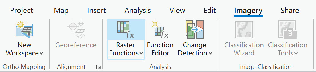
Figure 19.1. Selecting Raster Functions

Click the down arrow to find two options – Raster Functions and History (Figure 19.2).

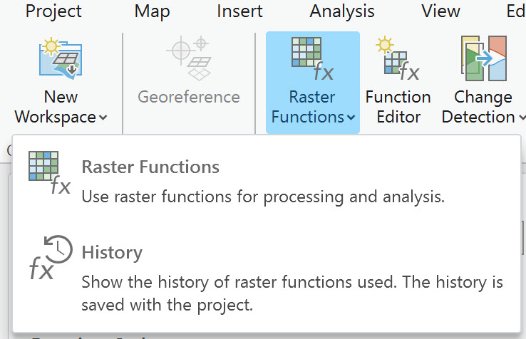
Figure 19.2. Raster functions options

Select Raster Functions. The Raster Functions pane lists several tools in the expanded Analysis category (Figure 19.3). Many of these are also available from the Geoprocessing pane.

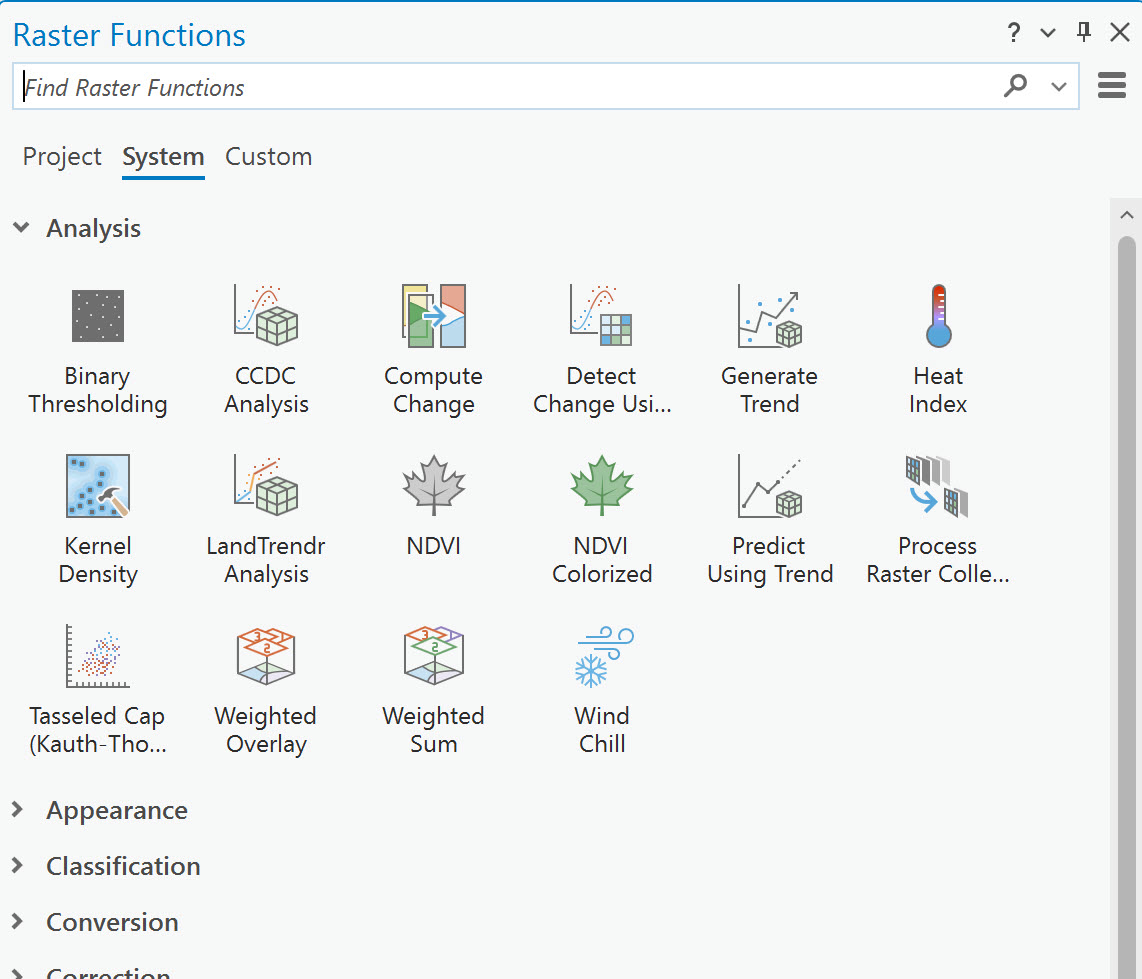
Figure 19.3. Raster functions

Additional categories can be expanded to show more processing function tools. In Figure 19.4, Math has been expanded. For example, individual Math tools are Abs, Divide, and Minus, and they are used with single-band images. The third tool in the first row is Band Arithmetic, used with multi-band images.

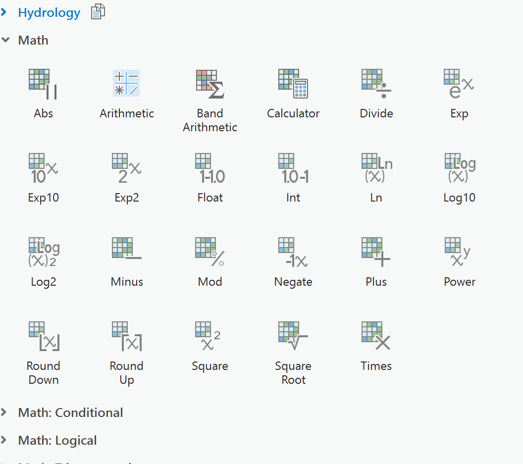
Figure 19.4. Expanding additional function tools

Select Band Arithmetic. The default Method is NDVI (Figure 19.5) which we will discuss later.

Figure 19.5. Band artithmetic properties

Click the drop-down arrow under Method to view a list of available ratios (Figure 19.6). 

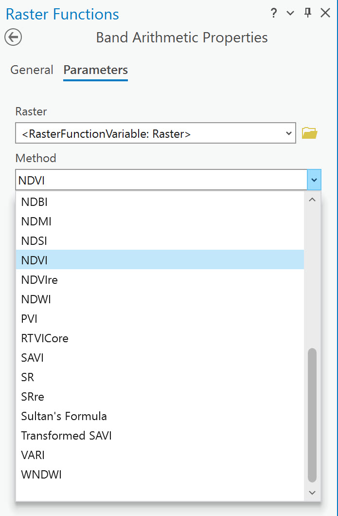
Figure 19.6. Band artithmetic properties

For simple band ratios, select User Defined at the top of the list (Figure 19.7).

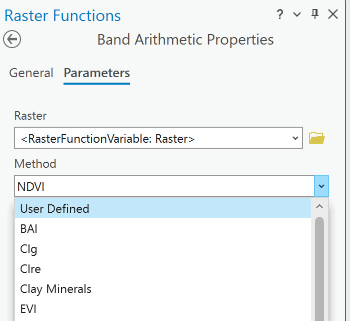
Figure 19.7. Ratios

Now we will create a NIR/Red Ratio to enhance the presence of vegetation.

Referring to Figure 19.8, select the composite image as the Raster. Under Band Indexes, we will enter the equation NIR/Red, but we need to remember that the band numbers associated with our image subset and assigned by ArcGIS^® Pro are B4 (NIR) and B3 (R). Be sure to include the parentheses when writing the equation as shown in Figure 19.8.

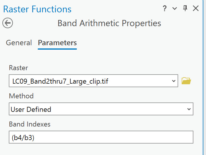
Figure 19.8. Parameters

Click on General and name the file. In Figure 19.9, we spelled out the word divide because special characters cannot be used when naming files. Additional details can be added under description, including metadata, to provide information on the process. Then click Create new layer at the bottom of the Raster Functions pane.

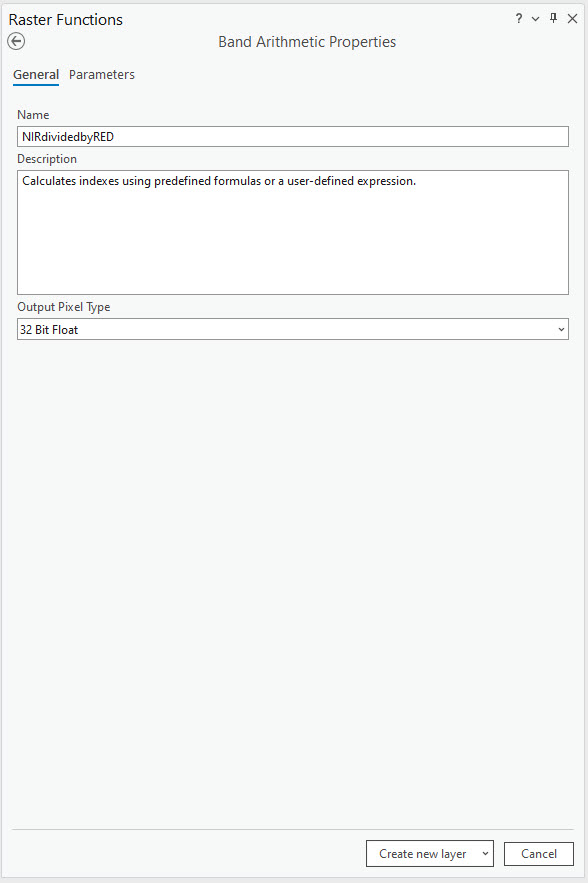
Figure 19.9. The raster functions pane

When complete, a green message temporarily displays at the top of the Raster Functions pane—”Band Arithmetic applied successfully”; a new layer shows in Contents and the Map viewer (Figure 19.10). Don’t worry if you don’t see the green message – it displays and disappears quickly. The process worked if you have the new layer.

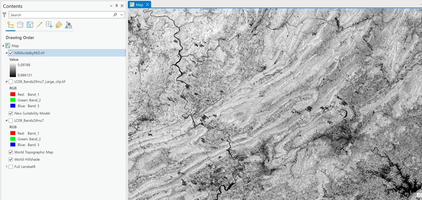
Figure 19.10. The map display

The brighter tones indicate denser vegetation. The symbology in Contents shows the higher value as the lighter color and the lower value as the darker color.

Can we confirm that the results showing brighter are denser vegetation? Use Swipe to compare the new image to the natural color composite (Figure 19.11). The brighter areas represent the forests, and some agriculture with vegetated fields, and the darker tones represent some fallow agriculture and developed areas.

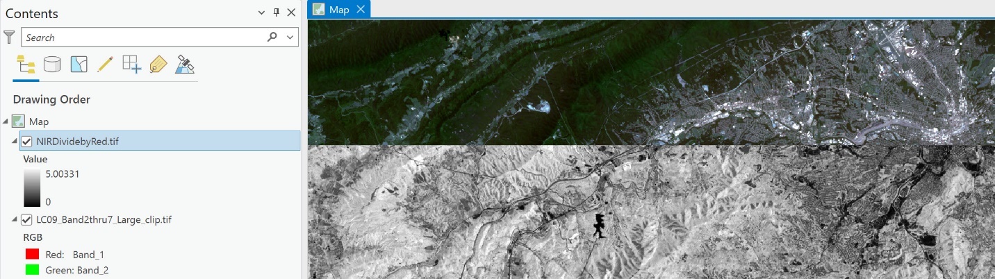
Figure 19.11. Using the swipe tool

In Figure 19.12, zoomed in to the City of Roanoke, the roads and river appear very dark. No vegetation is present in the dark areas.

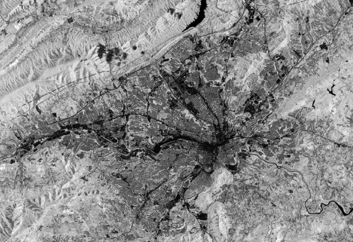
Figure 19.12 – Roanoke, Virginia, and Carvin’s Cove Reservoir (crescent-shaped water body in the north part of the image)

This process created a new image that shows as a layer in contents. However, this new image is present only in the current map project—no new data was created and saved. Once the tool has run successfully, the map project should be saved immediately. Tools in Raster Functions create an image useful for this map project only. This image cannot be used in another map project, and if the map project closes without being saved, the image will be lost.

Creating a Permanent Band Ratio Image using Geoprocessing Tools

We will repeat the process using a different method, which will create which will create new data saved in the geodatabase.

When using the Geoprocessing tools in the Analysis tab, ArcGIS^® Pro recognizes the pixel values for Landsat imagery as integers (whole numbers). So, the results are integers, usually rounded down when performing math operations. However, results for band ratios must be real numbers (numbers with decimal points). This means we must first change our image values to floating point values.

Go to the Analysis tab and select Tools. Under Find Tools, type Float. Select Float (Spatial Analyst Tools (Figure 19.13).

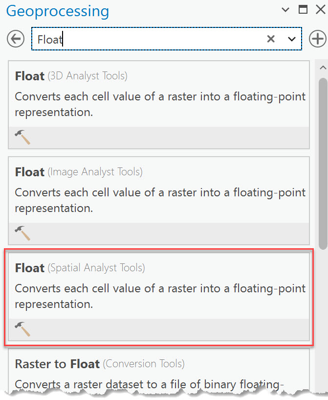
Figure 19.13. Float (spatial analyst tools)

This tool uses individual bands, not the composite image. So, the tool must be run twice, once for Band 5 (NIR) and once for Band 4 (Red). Remember that we are using the original bands we downloaded, so the band numbers in the file name correspond directly to the spectral channel. Either add these individual bands to the project or navigate to them using the file folder at the end of the Input Raster line. Then, run the tool twice, with the inputs shown in Figures 19.14 and 19.15. The results will include new image layers in Contents and two new images in the map viewer. Notice that we named each file appropriately.

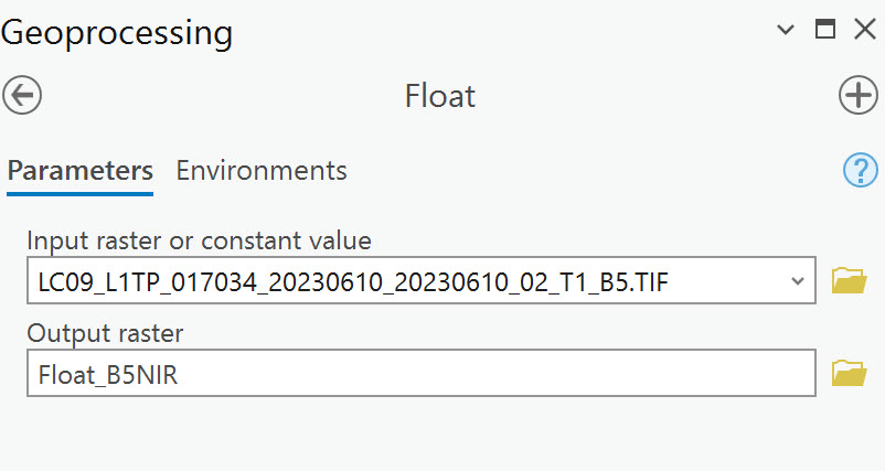
Figure 19.14. Float parameters

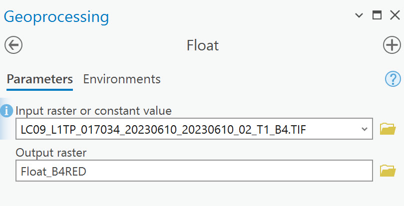
Figure 19.15. Float parameters

You will have two new layers in Contents and the Map viewer (Figure 19.16). The range of values is the same; the new files are values that are real numbers.

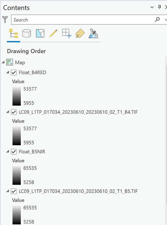
Figure 19.16. Contents

Now in Geoprocessing tools, search for the Divide spatial analyst tool, open it, and input the files as shown in Figure 19.17. Remember, the formula is NIR/Red. If you need help determining which image goes in which box, click on the information button at the beginning of the box. Name the Output Raster. Click Run.

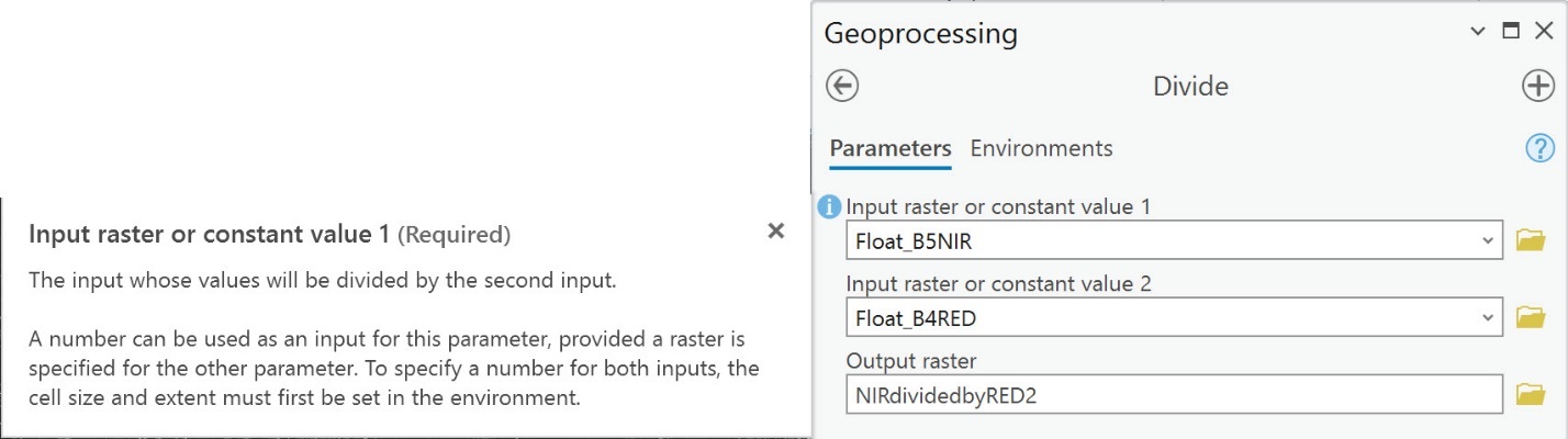
Figure 19.17. Geoprocessing: Divide

• When the tool finishes, the “Divide completed” message displays; point to the message, and a pop-out window opens that provides information on the process (Figure 19.18).

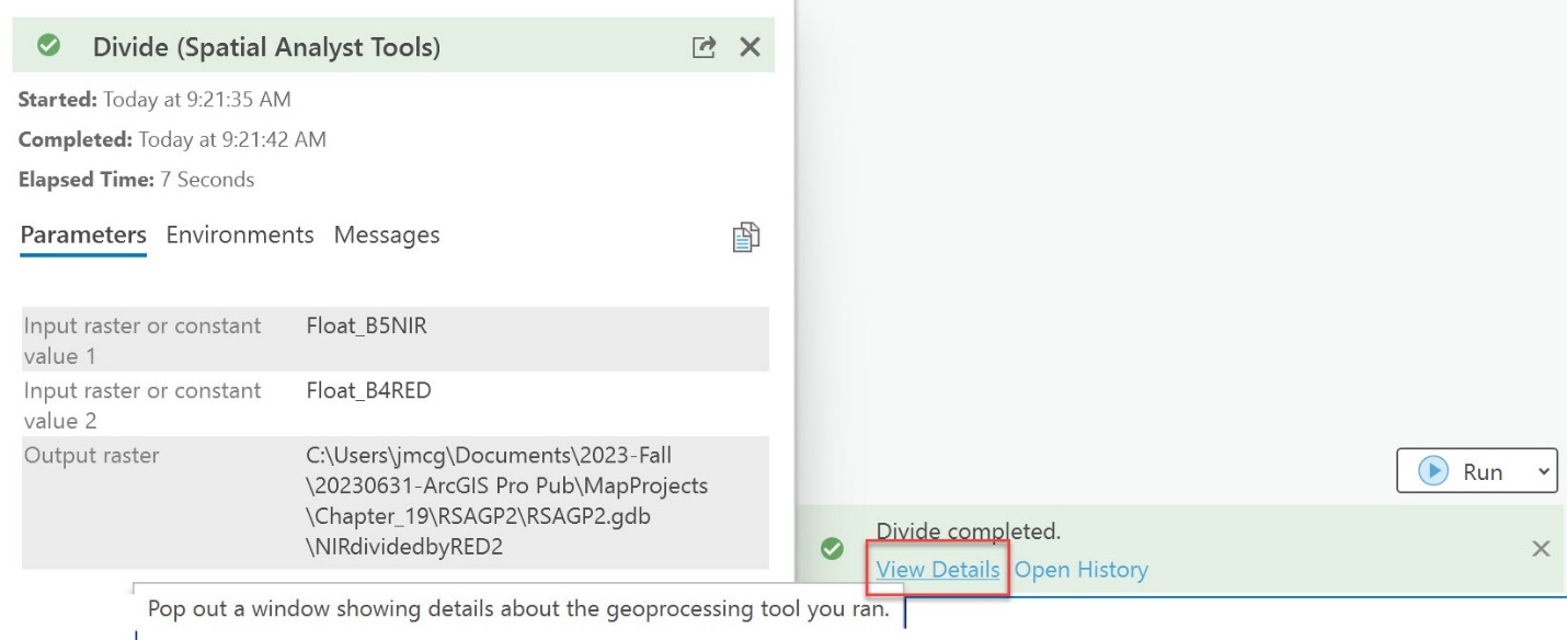
Figure 19.18. Divide (spatial analyst tools)

A new image layer is in Contents and the map viewer, but since we used the original single bands, it is the full extent of the Landsat scene (Figure 19.20). In addition, it appears in Contents that the image is not the same as the image that was created using the shortcut tool because the values have a wider range. But again, this is the full scene and not the subset used in the Raster Function process.

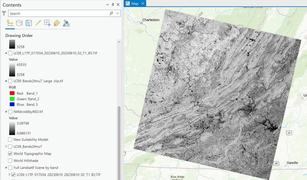
Figure 19.20. The full scene

To verify the results are the same, click on any pixel in the most recent new image. Examine the pixel value. In Figure 19.21, we zoomed in on the airport runway in Roanoke.

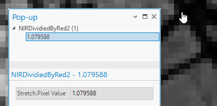
Figure 19.21. Zooming into the Roanoke airport runway

Now click on that same pixel in the image created using the Raster Functions shortcut (Figure 19.22).

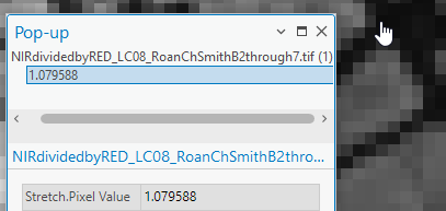
Figure 19.22 Selecting a pixel along the Roanoke airport runway

The pixel values from both methods used to create the ratio images are the same.

Now generate another ratio image 4 / 7 Ratio (Red/SWIR). This ratio is often used to identify differences in water turbidity. You can use either method outlined above, but if using the Geoprocessing tools, don’t forget to modify the floating-point image for each band. And remember, the Geoprocessing tools create a new image that can be used in other projects.

For demonstration purposes, we are using the Raster Functions > Band Arithmetic (Figure 19.23).

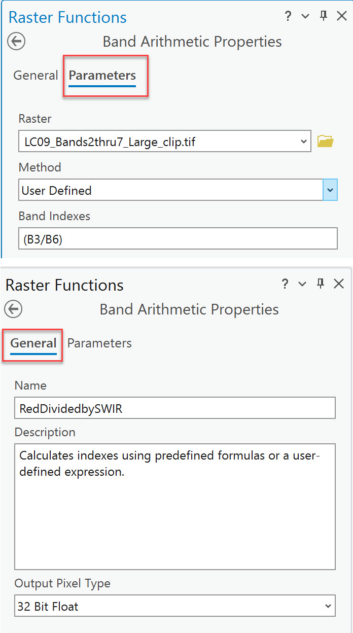
Figure 19.23. Raster functions

A new image layer is in Contents and the map viewer (Figure 19.24).

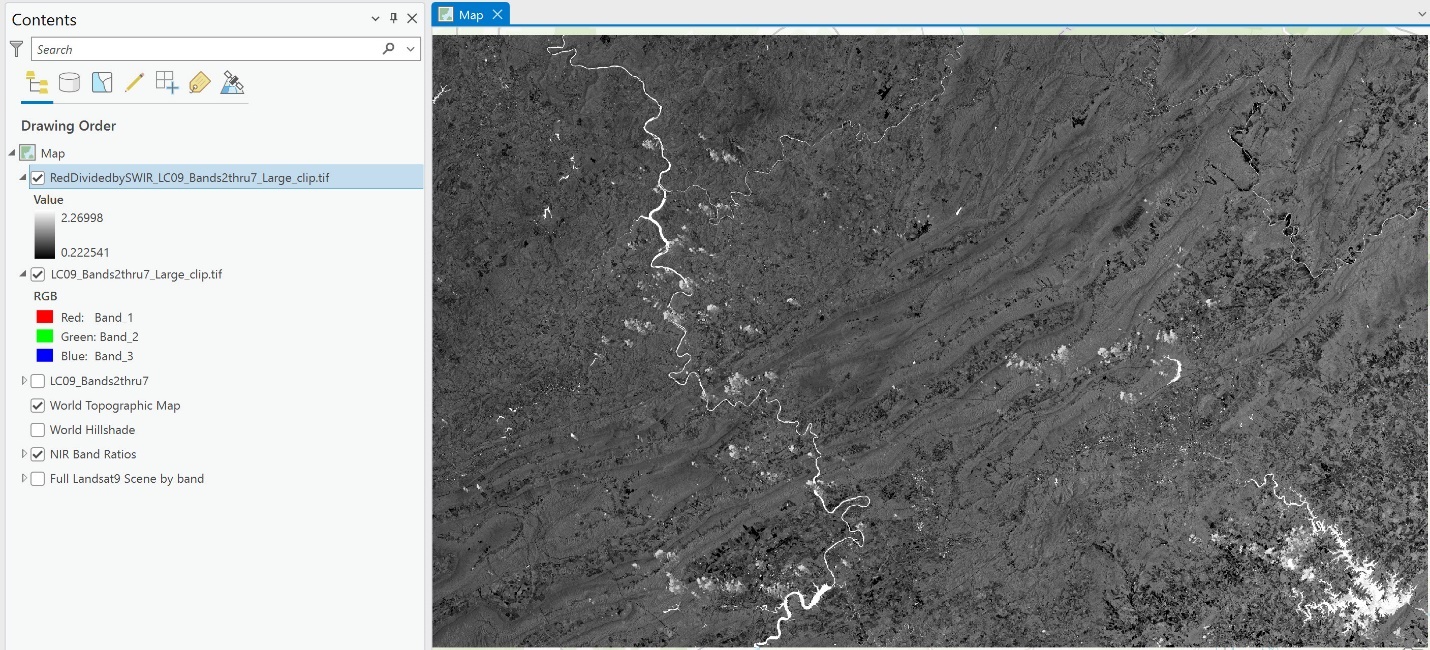
Figure 19.24. A new image in Contents

Areas of water are very bright. The New River located to the west (left), Smith Mountain Lake in the southeast, and Carvin’s Cove in the central portion of the image are very prominent, as are other individual water bodies scattered throughout the image. This band ratio shows water turbidity, so let’s zoom into Smith Mountain Lake, located in the southeast corner of the image (Figure 19.25).

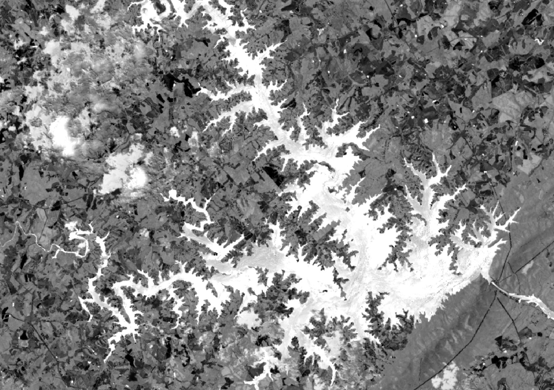
Figure 19.25. Smith Mountain Lake

While most of the lake is very bright white, dark areas are apparent in the southeast, where the lake drains into the river, as well as in the northwest branch. Using the Swipe tool, let’s compare it to the natural color composite (Figure 19.26).

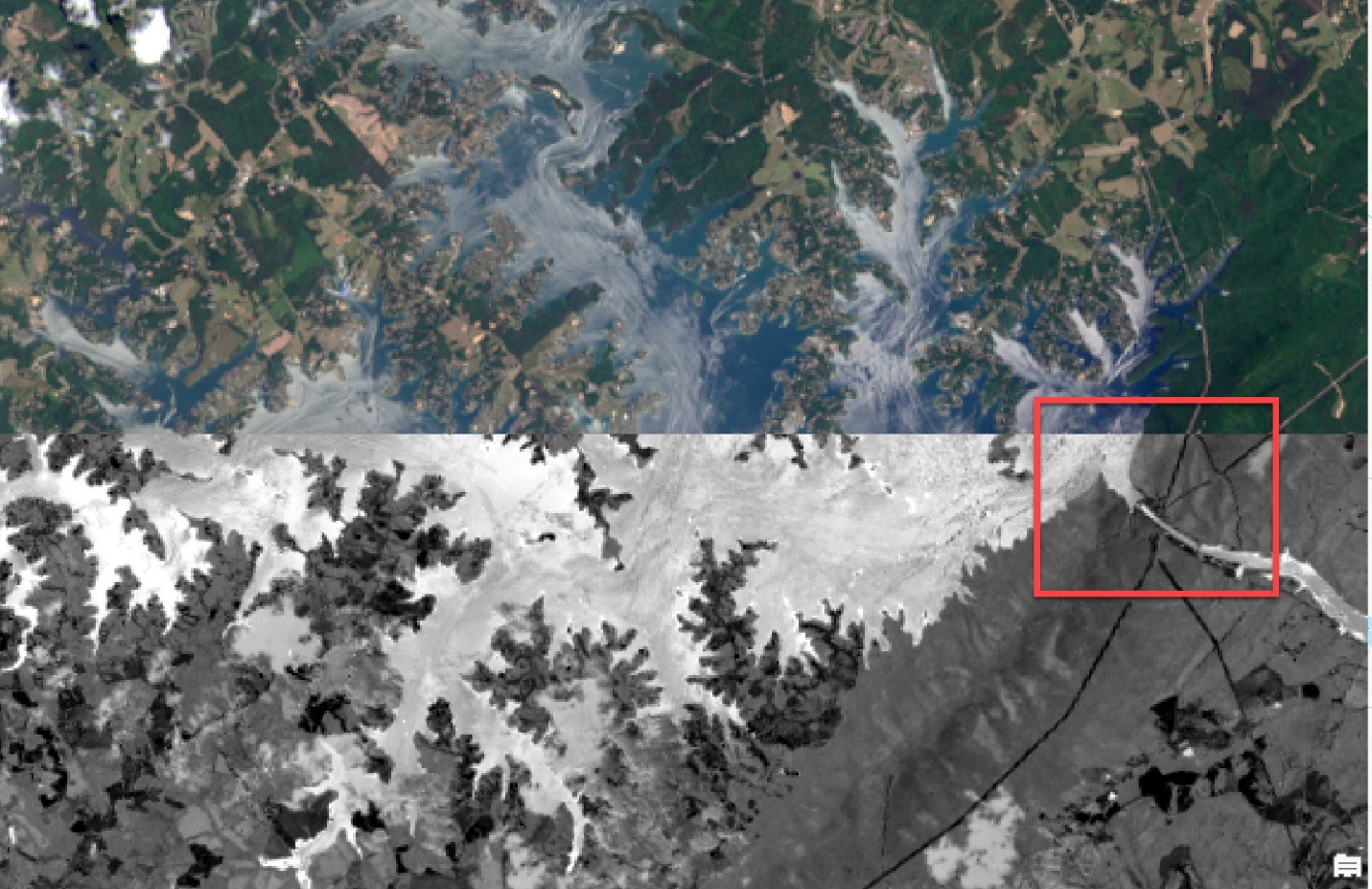
Figure 19.26. Using the swipe tool

What do you see? Why would areas leading into the lake be brighter? This river runs through a city and some agricultural areas, so it is experiencing runoff, which makes the water more turbid and sediment-filled, so brighter pixel values in the natural color image and a bit darker in the ratio image. What about the dam area shown in the red box? The areas right above and right below the dam are more turbid because the water is funneled through the dam’s turbines, thus flowing more rapidly than the areas farther north and west.

Any simple ratio can be accomplished with these methods. And more complex ratios can also be accomplished using these tools, but ArcGIS^® Pro has some shortcut tools. The Raster calculator in Geoprocessing/Spatial Analyst allows calculation in one step. We will explore these with indices in the next section.

Vegetation Indices

Vegetation indices are another form of spectral image transformation. This section discusses three: NIR/R, square root (NIR/R), and NDVI.

IR/R was already calculated above (5/4 ratio). For Landsat 9, Band 5 was NIR, and Band 4 was Red. This ratio can also be calculated for other sensors; ensure NIR and Red bands are used and not the band number. For example, for Landsat 7 ETM+, Band 4 is NIR, and Band 3 is red. And remember, if your composite image is not a composite of all bands, ArcGIS^® Pro will renumber them!

Let’s look at the square root of IR/R next. Since we already have NIR/Red, we only need to run a tool that calculates the square root.

Go to the Imagery tab, Raster Functions > Math, and select Square Root (Figure 19.27).

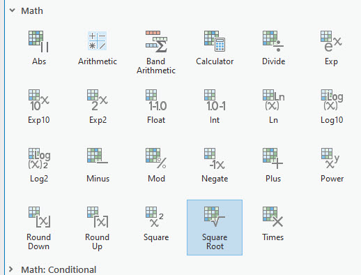
Figure 19.27. Raster functions

Choose one of the 5/4 ratio images created above. It does not matter which one; we selected the one created using the Geoprocessing tools. Remember to name the new layer under the General tab. Leave all the other settings as default (Figure 19.28).

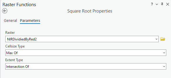
Figure 19.28. Square root properties

We have generated a new image (Figure 19.29). Because we used the one created with the Geoprocessing tools, it reaches the extent of the entire Landsat scene. And since we used Raster Functions, the image exists only for this map project.

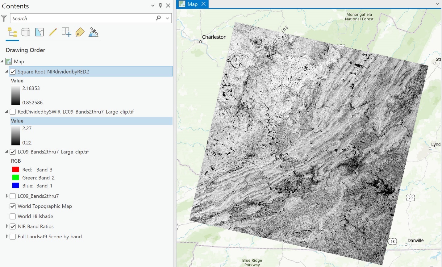
Figure 19.29. The map display

You can rerun the process using the Geoprocessing tools. We will not demonstrate it here. Just remember, using the Geoprocessing tools creates a new image that can be used in other analyses.

Now, what exactly did this index show? Zoom in on the mountain area around Carvin’s Cove. Adding the square root function makes the image slightly brighter and provides a sharper distinction between features compared to the NIR/RED ratio (Figure 19.30, red arrow points at the swipe line).

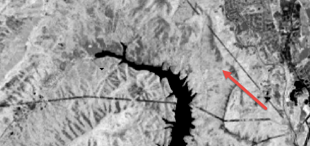
Figure 19.30. Comparing images using the swipe tool

Above, we demonstrated a step-by-step method to generate an enhanced image using an index. It is possible to do this using Raster Calculator in just one equation. Float can also be calculated within this single equation, but we will not do that since we already have the float images. Use of the Raster Calculator tool requires special attention to building the equation.

Go to the Analysis tab, Tools, and search for the Raster Calculator (Spatial Analyst Tools) (Figure 19.31).

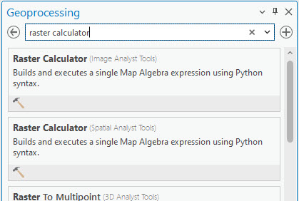
Figure 19.31. The raster calculator

The tool should be populated as follows. Double-click to choose the image from the list on the left and the operator from the tools on the right. Note that your formal names may differ slightly from the example below, since the ratios layers have been organized and placed into a “NIR Band Ratios” group in Contents. 

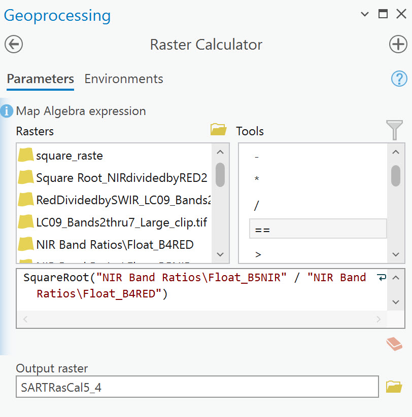
Figure 19.32. A raster calculation

Figure 19.33 shows the result. There is no difference between the two methods except for the number of steps. Also, remember that a new image is generated using the Raster Calculator and is available for other map projects. Again, to demonstrate no difference in the results between the two methods, we will look at a pixel value from an island in the New River by Radford, Virginia. For the general location, see the yellow oval in Figure 19.33. For the specific pixels, see Figures 19.34 and 19.35.

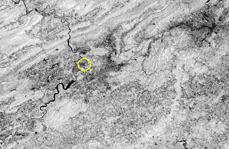
Figure 19.33. General location in the image

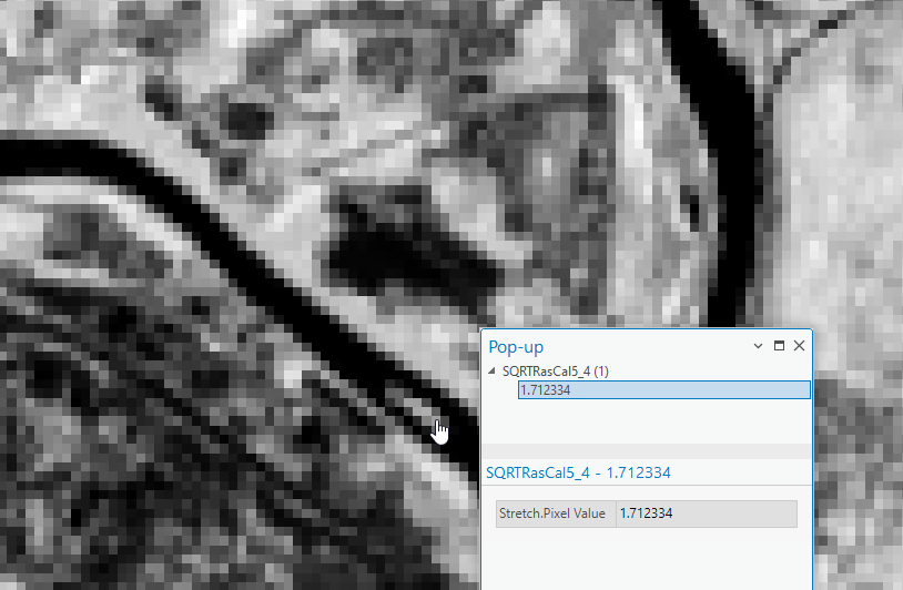
Figure 19.34. Selecting a pixel

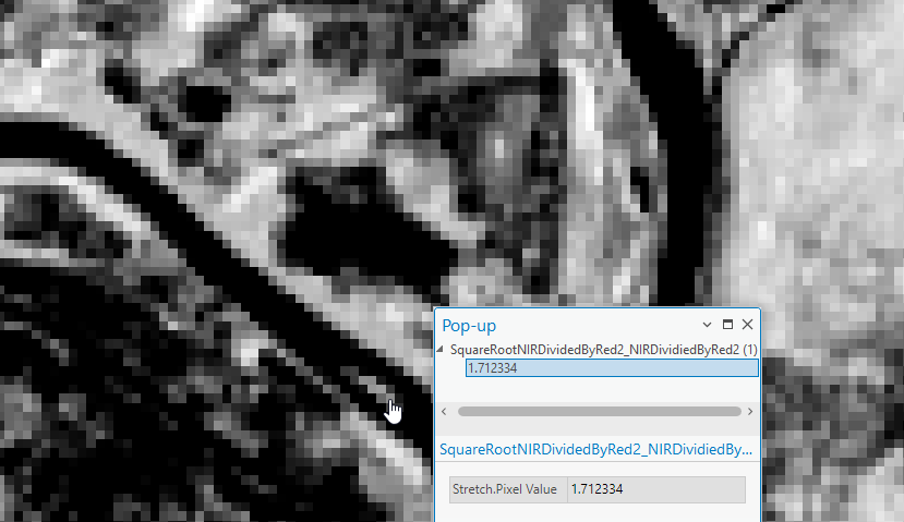
Figure 19.35. Selecting a pixel

Calculating Normalized Difference Vegetation Index

The Normalized Difference Vegetation Index (NDVI) is an important and the most commonly used vegetative index. Healthy green leaves have a higher reflectivity in the near-infrared band, while stressed, dry, or diseased vegetation display lower levels of reflectivity. NDVI can therefore be useful as an indicator of vegetation stress. It is a more complex calculation. The formula for NDVI is:

NIR-R/NIR+R or for Landsat 9, B5-B4/B5+B4

Open the Raster Calculator. If the original Landsat bands (5 and 4) are not present in the current map project, use the Add Rasters folder to navigate to and select them. When selected, they are added to the Rasters list in Raster Calculator but not added to the map project.

We now need to build the equation carefully. Typical mathematical order of operations applies. It is essential to place parentheses correctly. Otherwise, the Raster Calculator tool will perform the operation from left to right with an incorrect result. The equation should look like this:

(NIR – Red) / (NIR + Red) (Figure 19.36).

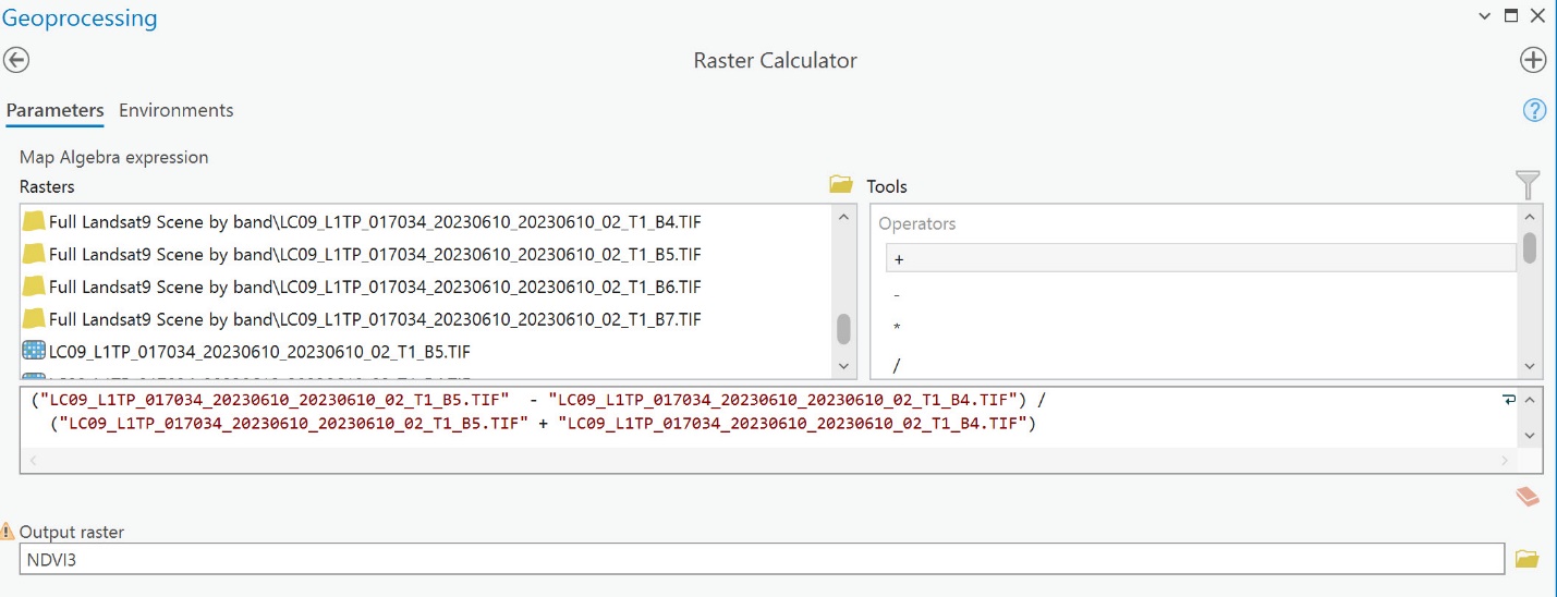
Figure 19.36. NDVI formula

Do not type the band number; instead, double-click the specific image bands from the list on the Rasters side of the Raster Calculator pane.

Here is the process for building the expression:

• Type an open parenthesis (.
• Select(double-click) the NIR band 5 from the Rasters list.
• Select (double-click or type) the minus sign from the Tools list on the right.
• Select the red band from the list.
• Type a closing parenthesis ).
• Select the division sign /.
• Type another open parenthesis (.
• Select the NIR Band.
• Select the plus sign.
• Choose the red band.
• And finally, type the closing parenthesis ).

Once the equation is written correctly, select Run.

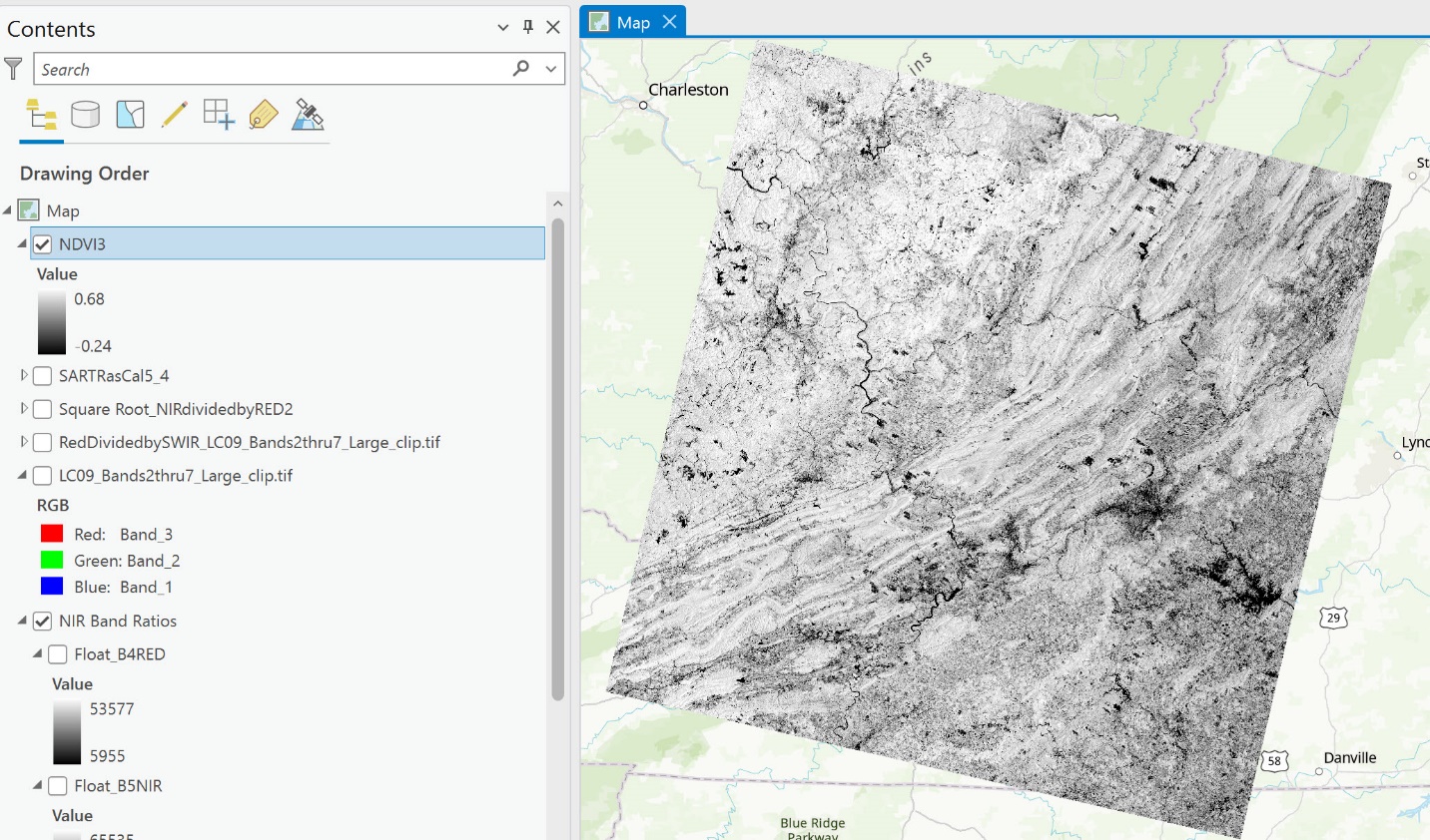
Figure 19.37. NDVI image

The NDVI result gives pixel values ranging from -1 to +1. The closer to +1, the brighter the pixel. Higher pixel values are associated with more vigorous or healthier vegetation. For this image, the brightness values only range from -0.24 to +0.68 because we do not have any values at the absolute ends of the range.

But guess what? There is an easier and much simpler way to generate an NDVI image in ArcGIS^® Pro! However, there is a catch — the NDVI image created from these other options is only available in the current map project.

The NDVI Shortcut tool in ArcGIS® Pro

We are going back to the Raster Functions under the Imagery tab. The third and fourth icons in the second row of the Analysis category are NDVI and NDVI Colorized (Figure 19.38).

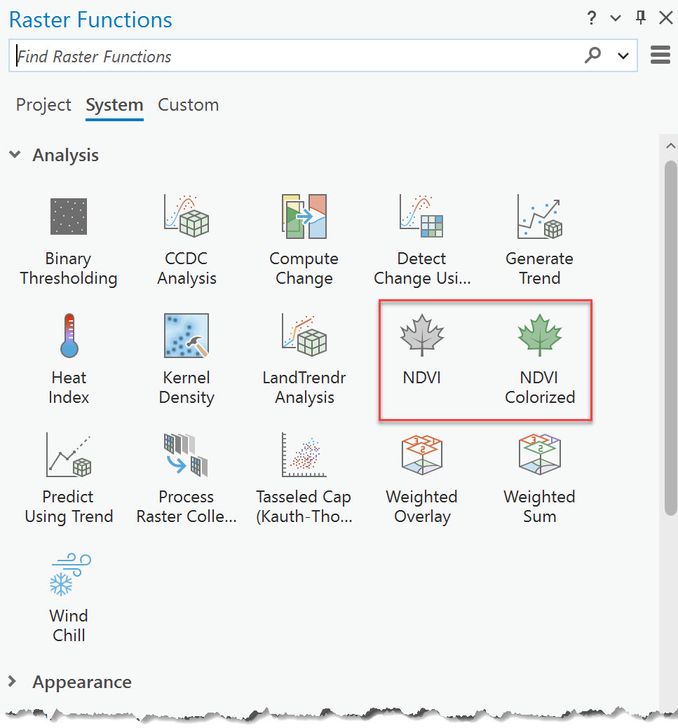
Figure 19.38. NDVI shortcut in Raster Functions

Select NDVI and the NDVI Properties tool opens (Figure 19.39).

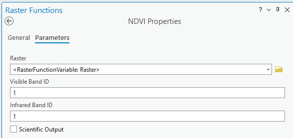
Figure 19.39. NDVI properties

The Raster is the composite image. Then choose the appropriate band number for Visible Band ID and Infrared Band ID. Check the box for Scientific Output. (Figure 19.40). Then select Create New Layer. Remember, since our Landsat composite image does not include band 1, this impacts our Landsat band sequence.

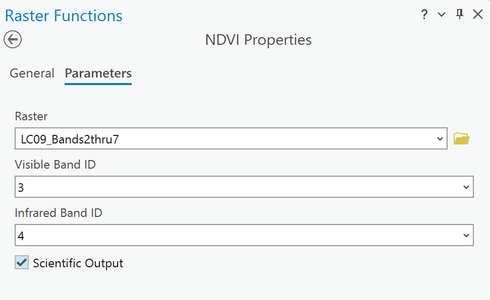
Figure 19.40. NDVI Properties

The results are shown in Figure 19.41. The Raster Calculator generated image values that are from -0.24 to +0.68. Using this shortcut tool, a different range of values is -0.186148 to +0.672007. What is the difference? Remember, the first NDVI image was created with the entire scene extent; this one was created from the subsetted multi-band image. Your symbology may be different from what is shown.

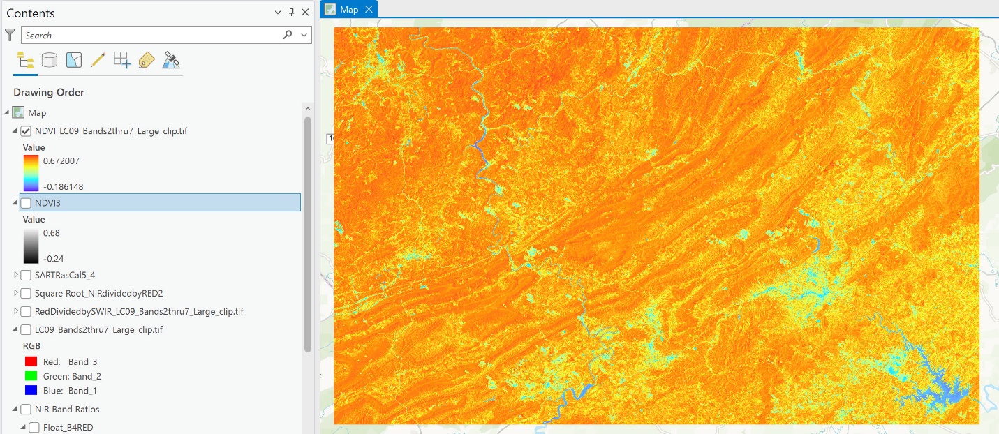
Figure 19.41. NDVI image

Additionally, the image created with this tool is only available for use in this map project. So, quickly save the project so the image is preserved!

There is one additional method under Raster Functions; an NDVI Colorized option is available. This generates a color map or color ramp to display the output. 

Go back to Raster Functions and open the NDVI Colorized tool. Enter the parameters as shown in Figure 19.42. Then click on Create a new layer.

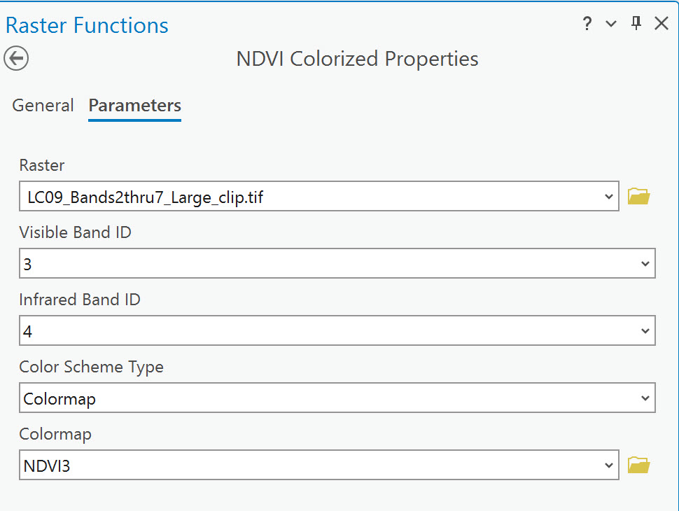
Figure 19.42 NDVI colorized properties

The figure below shows the results with colorized pixels and no Scientific Output. The image in the map viewer is colorized, but the pixel values in the Contents are integers, not real numbers. With NDVI, the values of the pixels should range from -1 to +1, not values over 1 (Figure 19.43).

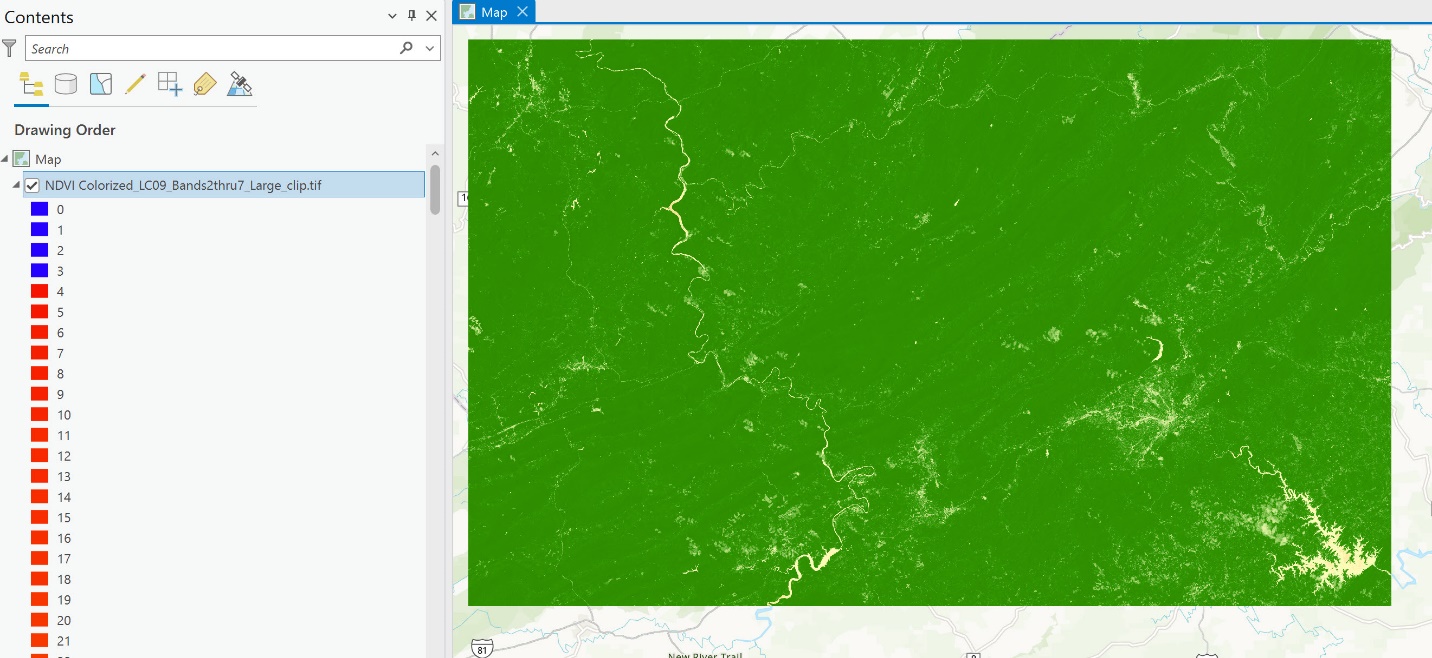
Figure 19.43. NDVI class values

If you need a specific colorized version of NDVI, create the index using the Geoprocessing tools and then change the symbology.

An alternative to creating an NDVI image is available. See https://www.usgs.gov/landsat-missions/landsat-surface-reflectance.

Surface Reflectance products, including NDVI, can be ordered as on-demand products; they cannot be directly downloaded. Go to https://espa.cr.usgs.gov/ . The login should be the same as for Earth Explorer. The authors believe there is tremendous value in learning to generate image-derived products using Spectral Enhancement techniques and not solely relying on pre-processed products.

When we first introduced Raster Functions> Band Arithmetic, the default was NDVI, but under Method was a list of additional indices (Figure 19.44 shows the entire list).

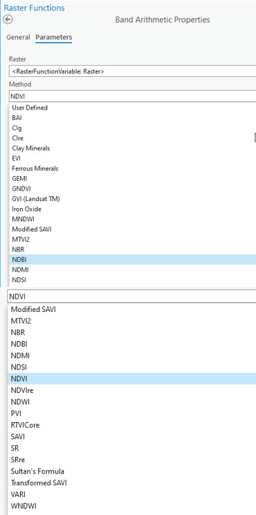
Figure 19.44. Other indices

Each one of these indices has been vetted within academic research and literature. These should be reviewed for specific applications. For definitions of the additional ratios available under Raster Functions methods, see http://pro.arcgis.com/en/pro-app/help/data/imagery/band-arithmetic-function.htm.

Please note that any spectral band index can be created within ArcGIS^® Pro using the raster calculator and manually typing the equation or with several steps using the map algebra tools identified above.

Summary

Within the last three chapters, we demonstrated the image enhancement processes. These processes are helpful for image analysis and for completing additional processing, such as image classifications discussed in Chapters 21 through 24.

The next chapter of this book, Chapter 20: Change Detection, will require downloading two additional Landsat 9 scenes, so be prepared to review and utilize skills acquired in Chapters 11, 13, and 15.