20 Chapter 20: Change Detection using Landsat 9 Imagery

Introduction

Remotely sensed imagery is useful in detecting changes in features on the surface of the Earth. To detect changes in land use and land cover, imagery is required, usually from the same sensor and from two different dates. Change detection aims to identify changes in the spectral properties of specific features (pixels) associated with these two dates. The interval between dates can be as short as a few days, for example, to detect impacts of natural disasters, a few months to assess growth in large agricultural fields, or a few to several years to monitor changes in forest extent. Such analyses are called Change Detection.

Changing spectral properties of surface features provides information on effects such as land use changes (conversion from forest to urban), expanding urban areas (urban to urban comparison), effects of natural disasters (such as hurricanes and wildland fires), or impacts of insect infestations on forest cover. Change detection applies algorithms specifically designed to detect meaningful changes, in contrast to image differences originating in ephemeral (or superficial) features that do not signify meaningful differences over time.

A critical first step in a change detection analysis is identifying and selecting suitable pairs of images acquired over the same region. First, the two images must register either to each other or to the surface of the Earth—the region they cover must match exactly when superimposed. Second, the images must be acquired during the same season to track long-term changes, such as deforestation. Finally, it is vital that no significant atmospheric effects have impacted an image. The two images must be compatible in almost every respect, including but not limited to scale, geometry, and resolution. Otherwise, the change detection algorithm interprets incidental differences in image characteristics as genuine landscape changes.

Many alternative change detection algorithms exist and have been evaluated. Two main change detection approaches are pre-classification and post-classification. Image classification is discussed in Chapters 21 – 24. Pre-classification change detection examines differences in two images before any classification process. Post-classification change detection defines changes by comparing pixels in a pair of classified images in which pixels have already been assigned to classes. Post-classification change detection typically reports changes as a summary, a difference in digital numbers, of the from-to changes of categories between two dates.

This chapter introduces a simple procedure of pre-classification change detection using one band from each date and calculating differences in pixel values between these two dates to evaluate changes. More complex approaches, such as those involving PCA analysis or changes, are available when comparing two images processed with spectral indices such as NDVI. Still, these are beyond the scope of this book. This chapter also relies on knowledge gained from Chapters 11 and 13 through 19. You will be expected to apply several processes from those chapters. The specific chapter is referenced when a particular process is needed.

Change Detection: Getting Prepared

During our discussion of change detection analysis, two images acquired over southwestern Colorado will be used to evaluate landscape changes from drought and wildland fire.

On June 1, 2018, a fire started in the San Juan National Forest of southwest Colorado. The cause of the fire remains unknown. This fire was named the “416 Fire”. As of June 21, 2018, the fire had destroyed over 34,000 acres of forest and was only 35% contained.  The extensive nature of the fire, and the inability to contain it, was directly related to recent drought conditions in Colorado. NOAA had deemed this region to be in an exceptional drought. A typical annual snowfall for this region is approximately 71 inches. However, in the 2017/2018 winter season, snowfall was 65% less than average. Local snowpack, typically present in June, was gone by June 2018.

Download two Landsat images (Landsat 8) for this region before proceeding. The images are Path 35, and Row 34, with June 15, 2017, and June 18, 2018 dates. Follow the instructions in Chapters 11 and 13. Earth Explorer provides results in reverse chronological order—most recent dates are displayed first. The two images needed are identified in Figure 20.1. The lack of snow cover is evident in the June 18, 2018, image compared to the June 15, 2017, image (white circle). Note that in this exercise, we are working with Landsat 8 images, but the process is exactly the same using Landsat 9.

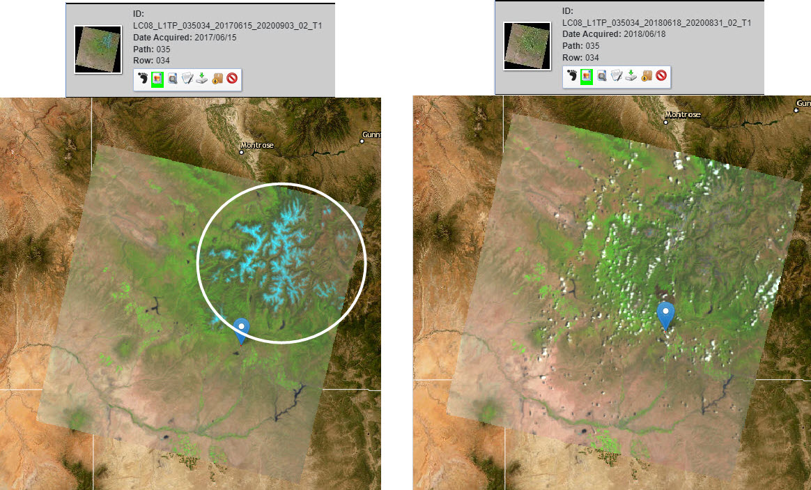
Figure 20.1 Note the difference in snowpack between the June 15, 2017 image (left) and the June 18, 2017 image (right) as captured by Landsat 8 as viewed in the USGS’s Earth Explorer

Since Earth Explorer provides the option to select which bands to download, only download Band 5 for each date (Figure 20.2).

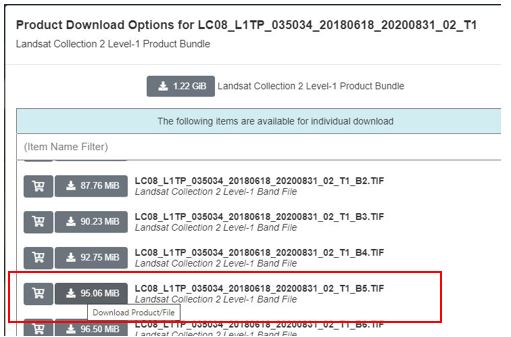
Figure 20.2. Downloading Band 5

The Change Detection Process

As with processes demonstrated in Chapters 15, 18, and 19, ArcGIS^® Pro provides multiple methods to conduct change detection. This section of this chapter will show a step-by-step change detection method. Then, we will give the change detection results produced using two other methods—Raster Functions and Raster Calculator. Students must refer to the prior chapters if a refresher is needed to locate those methods.

Change detection means applying image differencing, subtracting corresponding pixel values at each pixel, and then displaying the differences as colors, so the areas that differ in brightness can be easily identified. To generate useful results, the analyst must understand the region represented in the image and the subject of the analysis. Here, we will not use the composite image to calculate the differences, so it is essential that you know which Landsat bands are best suited for distinguishing which features. So why did we choose Band 5? Recall the discussion of bands that are useful for each analysis (Figure 20.3) or visit https://www.usgs.gov/faqs/what-are-band-designations-landsat-satellites .

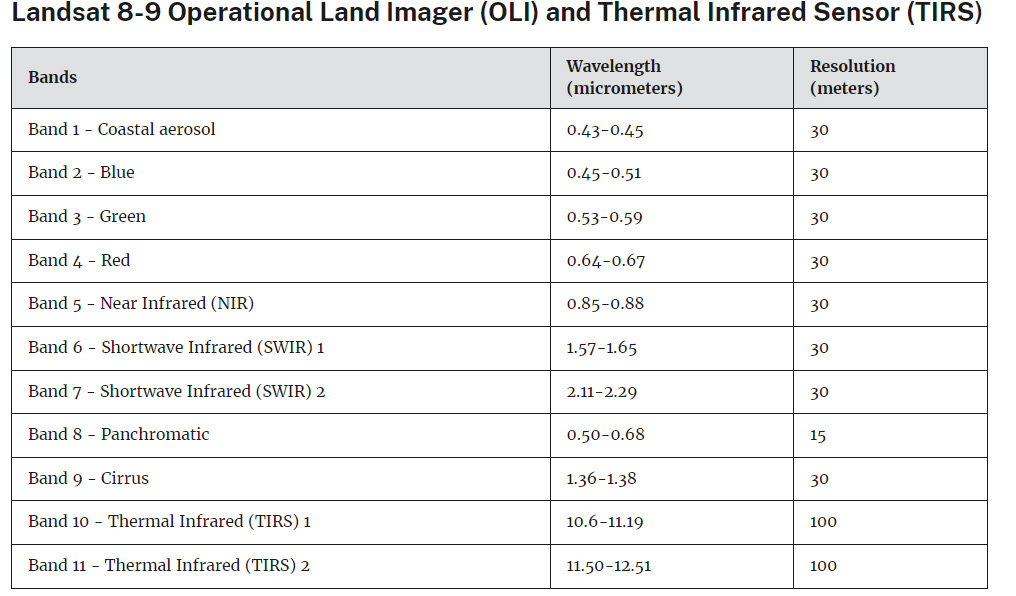
Figure 20.3. Landsat 8/9 spatial and spectral properties. Source: USGS (https://www.usgs.gov/faqs/what-are-band-designations-landsat-satellites)

A fire will significantly lower biomass. We will use Band 5 because, as indicated in the table above, Band 5, in the near infrared, emphasizes biomass content and supports the identification of shorelines. Shorelines discriminate between land and water, drought changes water body size, thus changing shorelines, and snow is just frozen water—all pertinent to our study. In addition, Band 5, as an infrared band, will experience little atmospheric scattering.

Change Detection Approach #1: Using the Change Detection Wizard

Open a new map project. Set the environments and workspaces. Before adding the images to your map, add them to the folder for your map project (Figure 20.4).

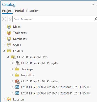
Figure 20.4. Adding images to your map project.

Add Band 5 for each date to your map project. Be sure that June 18, 2018, is the topmost layer in the Contents pane (Figure 20.5).

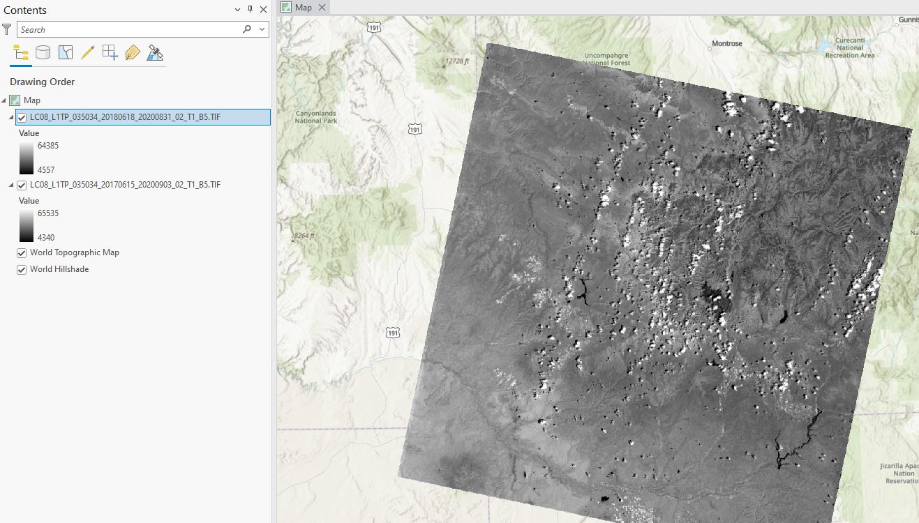
Figure 20.5. The Contents pane

First, select both layers in the Contents pane by holding down ctrl on the keyboard and clicking each layer. Under the Imagery tab, locate Change Detection (Figure 20.6)

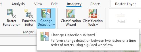
Figure 20.6. Selecting the Change Detection option

Click the button to open the Change Detection Wizard pane (Figure 20.7).

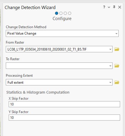
Figure 20.7. The Change Detection Wizard pane

There are several options (Figure 20.8). We are using Pixel Value Change which should be the default setting. Categorical change would be used if you were completing a post-classification change detection operation. Time Series Change would be used, for example, if you calculate the change in NDVI over a growing season.

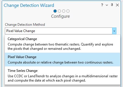
Figure 20.8. The Change Detection Wizard pane: Exploring options

The From Raster and To Raster can be in any order. You are calculating the difference between the two bands. In Figure 20.9, we have the earlier image as From Raster and the more recent image as the To Raster.

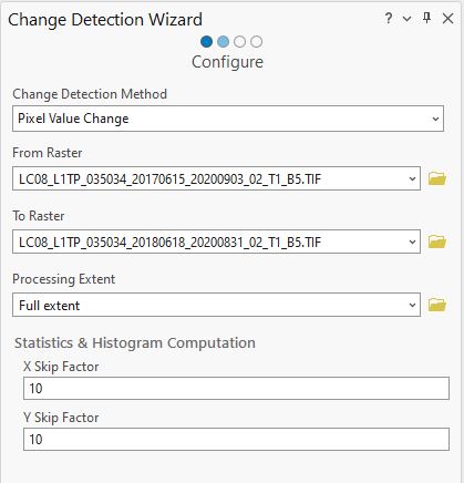
Figure 20.9. Configuring the Change Detection Wizard

Click Next at the bottom of the window, and page 2 of the wizard displays (Figure 20.10).

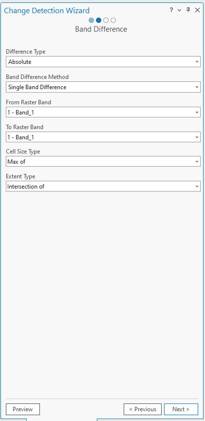
Figure 20.10. Configuring the Change Detection Wizard

There are additional settings that you can change. We want Absolute for the Difference Type. Our analysis uses single bands, so the following two settings show 1- Band_1. If we had a multiple-band image, we would want to choose, from a drop-down list, which bands we are using to calculate the difference. We are using the defaults for Cell Size Type and Extent Type as we want the difference between the entire images. At the bottom of the window are three buttons: Preview, Previous, and Next. The Preview button processes the change detection but creates a temporary image—a preview of what new image will be created. Previous goes back to the prior pane (Figure 20.9). Click Next. In this pane, we want to Compute Statistics & Histogram for the new image created (Figure 20.11). Click on that button.

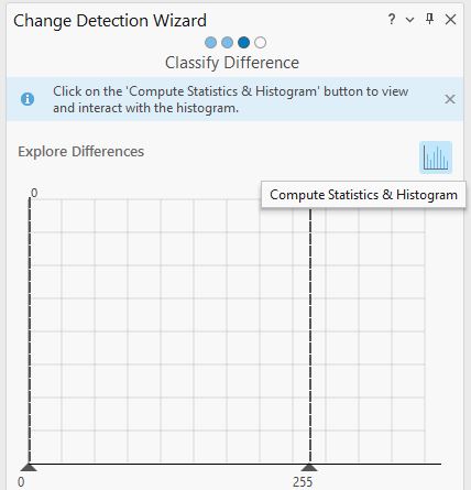
Figure 20.11. Computing statistics & histograms

You should now see a new image and the statistics and histogram for this new image (Figure 20.12).

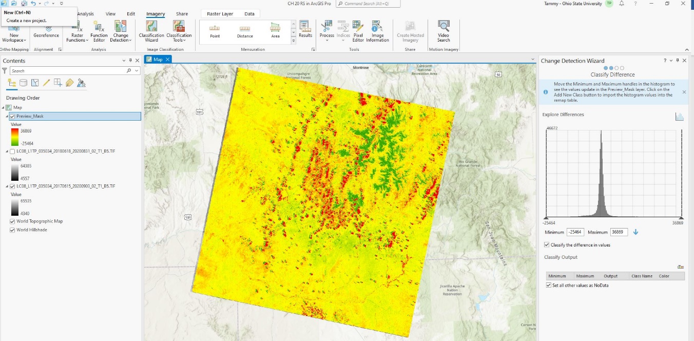
Figure 20.12. Image, histogram, and statistics for the new image

Don’t forget to SAVE your project!

What does this new image and the values in the Contents mean? The default symbology represents an increase in a pixel’s digital number. Red is an increase; Green means a decrease, and yellow means little or no change.

The June 18, 2018, image has clouds, and the June 15, 2017, image was cloud-free. The clouds are shown as red, one of the extremes in the change. When performing change detection, we recommend eliminating clouds. Change detection is used to monitor changes in the surface of the Earth. Clouds interfere with that process. For this exercise, the presence versus absence of clouds provides an excellent example of the change detection process.

What is the second most noticeable change? Snow cover. Snow was present in the mountains on June 15, 2017, but no snow was present in the June 18, 2018 image. Use the Swipe tool to compare the images (Figure 20.13).

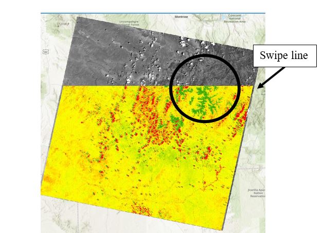
Figure 20.13. Using the Swipe tool

Let’s look at the image for other changes (Figure 20.14).

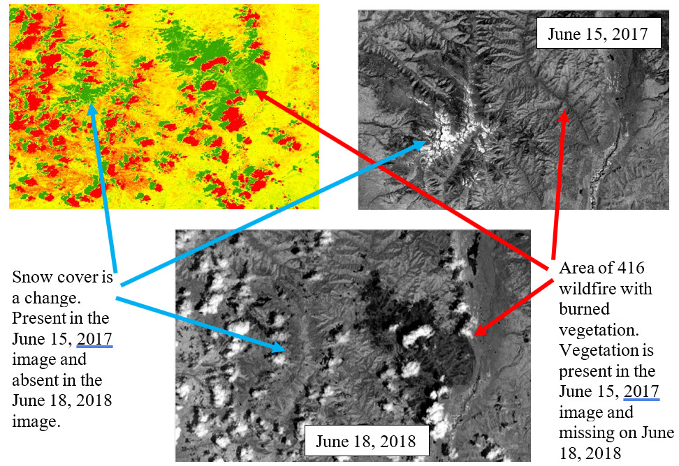
Figure 20.14. Comparing images

The lack of snow cover from the drought, and the lack of vegetation from the fire, both show a huge change in spectral values. Turn off the image created from the change detection, and let’s look at one more area of change; just to the east of the 416 Wildfire are two lakes (Figure 20.15).

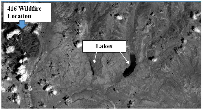
Figure 20.15. Exploring the impact of wildfire on local lakes

First, examine the two lakes, comparing June 15, 2017, image with the June 18, 2018 image (Figure 20.16).

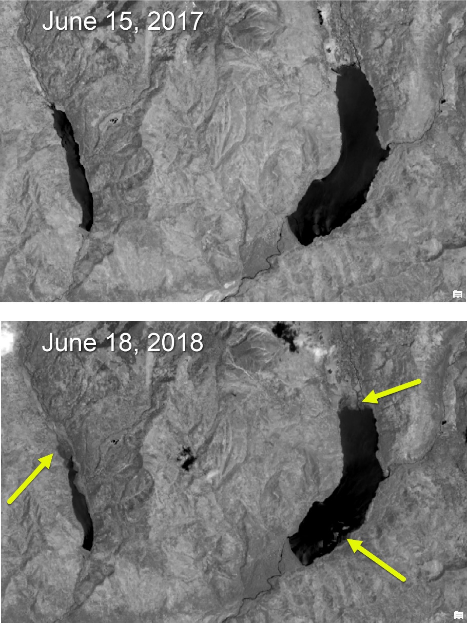
Figure 20.16. Exploring the impact of wildfire on local lakes

The changes in the black and white images in Figure 20.16, the original bands, are challenging to see. We are looking at the edges of the two lakes.

Now turn the change detection image back on. In Figure 20.17, look at the edges of the two lakes. The changes are noted in red, again, one of the extremes for the change in spectral values.

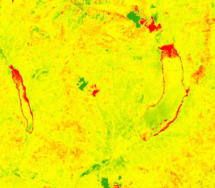
Figure 20.17. Change detection image of the two lakes.

The lakes in the June 18, 2018, image are smaller than the earlier June 15, 2017, image. Further, the shallow water in 2018 exposed sediment deposits concealed below the surface in 2017, as indicated by the green areas within the lakes. Also, remember that Band 5 is often used to discern shorelines.

Once a change detection process has been completed within ArcGIS^® Pro, it may be necessary to complete an image enhancement technique to discern the changes.

Suppose you are unsure what the original features represent when looking at a change detection image. In that case, it may be necessary to add a natural color or false-color composite image to the map project (reference Chapter 14: Creating a Composite Image using Landsat 9).

Thus far, we have completed a change detection analysis using the Imagery > Change Detection Wizard. Recall from prior chapters ArcGIS^® Pro provides several options to process functions.

Change Detection Approach #2: The Minus Tool

Use a Geoprocessing tool called Minus under Image Analyst Tools. Figures 20.18 and 20.19.

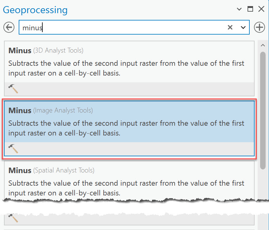
Figure 20.18. The Minus tool

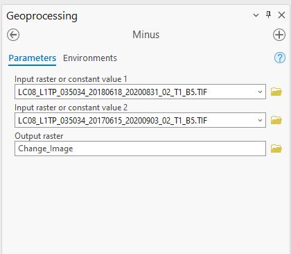
Figure 20.19. Running the Minus tool.

Our results appear to be different. Contents show a different range of values (Figure 20.20).

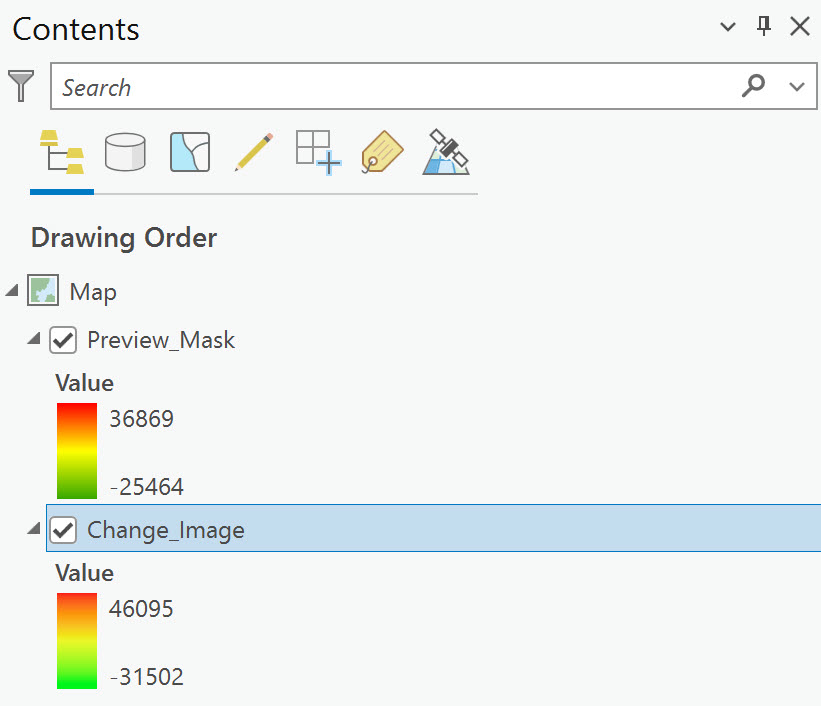
Figure 20.20. Comparing results

The range of values is different but are the individual pixels different? Zoom into the burn area and check individual pixel values (Figures 20.21 and 20.22). Be sure, when comparing, to select the same pixel from each image.

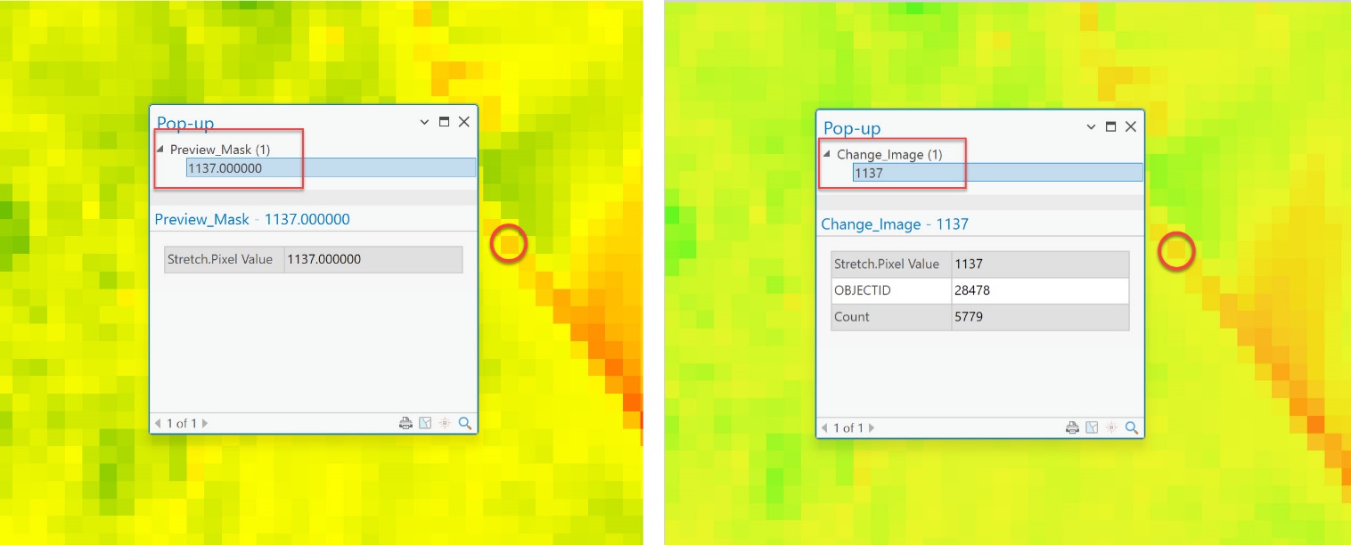
Figure 20.21. Comparing results

You likely can’t find the exact pixels used, but zoom in to any of the pixels in the burn area or the snowpack. Here is another example—zoom in to one of the lakes (Figure 20.23).

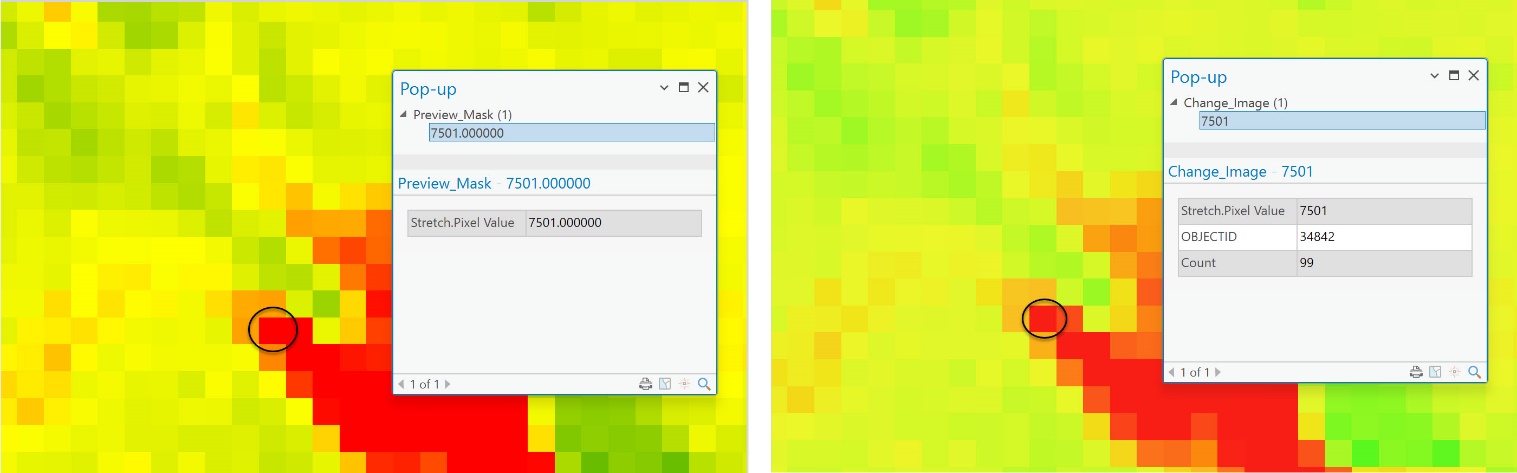
Figure 20.22. Comparing results

We now conclude the Change Detection process. Again, ArcGIS^® Pro provides many options for this processing, including methods discussed here and using Raster Calculator.

The band(s) selected for the change detection process will depend on the project’s goal and the exact features preferred for evaluating the change. This chapter addresses change detection only. These images of southwestern Colorado will not be used in any other chapter.