22 Chapter 22: Introduction to Supervised Classification of a Landsat 9 Image

Introduction

An analyst has more control over the supervised classification process than the software-controlled unsupervised classification process. Through supervised classification, the analyst selects pixels representing recognized landscape features/patterns or pixels that can be identified from other sources, such as high-resolution aerial photos. Knowledge of the data, the classes desired, and the algorithm to be used is required before selecting training samples—samples of spectral values within the image which pertain to specific features/patterns. The analyst “trains” the software to identify pixels with similar characteristics by identifying patterns in the imagery and chooses the spectral classes for the informational classes, thus, supervising the classification process.

Supervised training requires a priori (already known) information about the data, such as:

• The information to be extracted, for example, vegetation type or land use.
• The classes most likely present in the image, for example, land cover types such as forest, water, bare earth or forest, agriculture and urban, or any combination of those.

In supervised classification, the analyst relies on pattern recognition skills and a priori knowledge to direct the software in determining the spectral criteria, or signatures, for data classification. The analyst selects training samples for each informational class by identifying spatial or spectral characteristics of the pixels to be classified. For example, knowledge about a spatial characteristic may be known through field observations, analysis of high-resolution aerial photography, or personal experience. Field data are considered the most accurate data about a study area. They should be collected for the same time period as the remotely sensed data so that the data corresponds as much as possible.

Nevertheless, all field data may not be completely accurate because of observation errors, instrument inaccuracies, and human shortcomings. ArcGIS^® Pro calculates statistics from the training sample pixels to create a parametric signature for each class.

Every pixel value cannot be assigned to an informational class, but training data identifies many values. For any unassigned pixels, the analyst chooses the algorithm the software will employ to assign them to specific classes. Additionally, some pixel values may fall into two classes, a situation discussed in Chapter 21 on unsupervised classification concerning water classification and mountain shadows. Different algorithms include but are not limited to minimum distance, maximum likelihood, and Mahalanobis’ Distance. Please see Campbell, Wynne, and Thomas (2023 – 6^th edition) for more information about supervised classification strategies.

Instructions on supervised classification are divided into three chapters. This chapter introduces the different classification schemes available within ArcGIS^® Pro and provides instruction on creating training samples to use in the classification.

Chapter 23 provides step-by-step instructions on how to evaluate the effectiveness of the training samples. Training samples must be evaluated before conducting the classification. Approaches should take the following into consideration:

• The spectral values for each class must be independent of each other, without overlap.
• The full range of spectral values for a specific class must be included to check for overtraining or too many training samples that duplicate each other.
• The training samples represent a normal distribution of values.
• The analyst should avoid selecting training data near the edges of parcels to avoid introducing mixed pixels into the training data.

The final supervised classification chapter (24) provides instructions on creating a signature file for the classification scheme and conducting the supervised classification.

Objectives

The three chapters should be completed in sequence, Chapter 22 first, Chapter 23 second, and then Chapter 24. Within these chapters, you will:

• Create training samples (Chapter 22).
• Use histograms, scatterplots, and statistics to evaluate normality, separability, and partitioning of training data (Chapter 23).
• Generate supervised signatures using training samples (Chapter 24).
• Perform a supervised classification on a Landsat 9 composite image (Chapter 24).

These chapters use the 6-band composite Landsat 9 image, clipped to the extent of the map viewer created in Chapter 15. We will be using the same informational classes that we used in the chapter on unsupervised classification (Chapter 21), so as a reminder, the classes are:

ArcGIS Pro: An Introduction to Classification Schemes and Methods

Please open a new blank map project, name it, save it, set your workspaces, and add the 6-Band Composite image created in Chapter 15. Eliminate the background values, if necessary, and set the composite image to a natural color band combination (Figure 22.1).

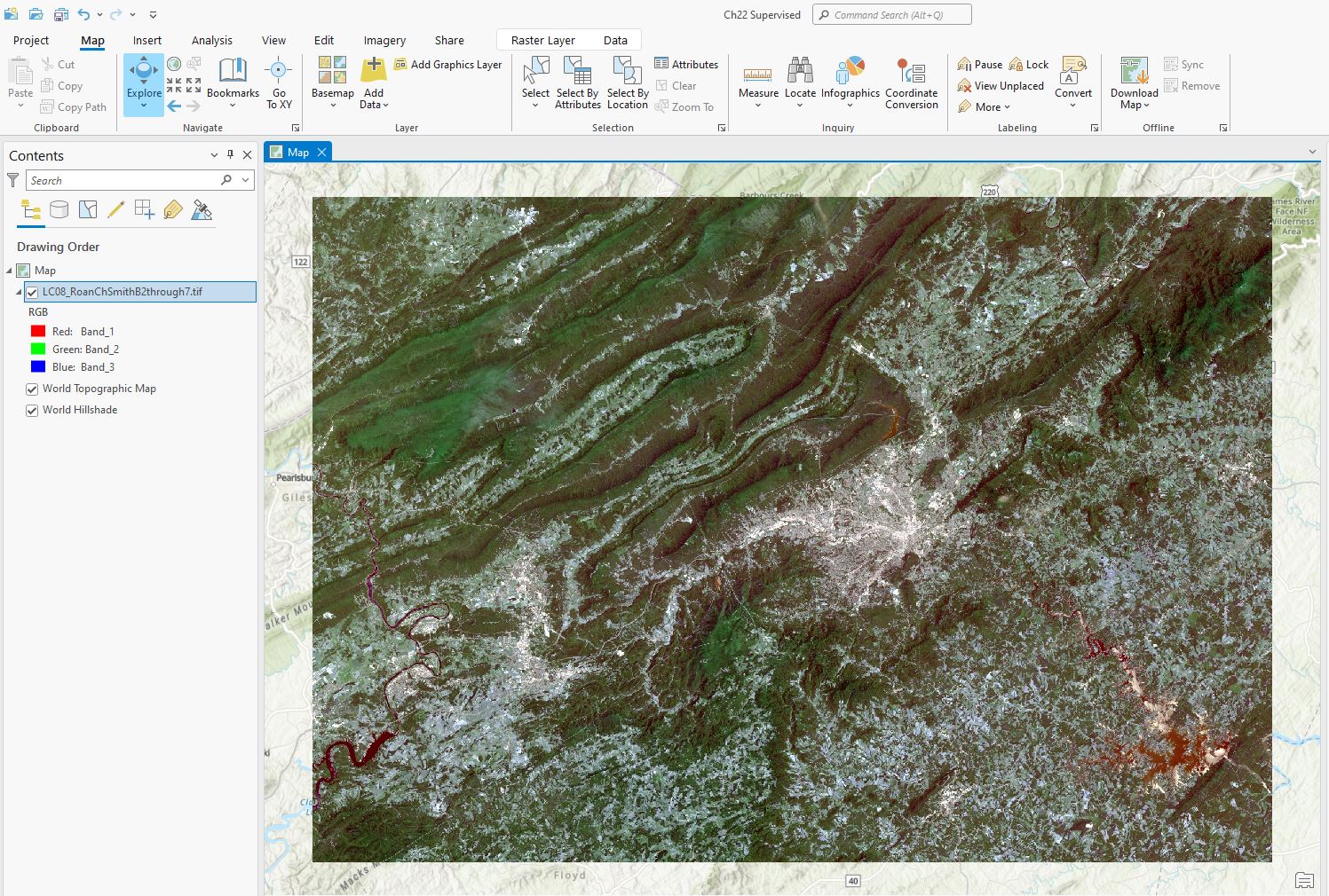
Figure 22.1 Setting the image to a natural color band combination

Before proceeding to the step-by-step process of supervised classification, we discuss alternative methods available in ArcGIS^® Pro.

The Image Classification Wizard

In Chapter 21, we identified the Image Classification Wizard under the Imagery tab on the ribbon. The Image Classification Wizard can perform both unsupervised and supervised classifications and combines several steps in the supervised classification process, bypassing many user prompts and decisions required with other software or processes within ArcGIS^® Pro.

Please note: it is unnecessary to follow along in ArcGIS® Pro at this juncture; we are just discussing the available methods.

The first choice to be made within the Image Classification Wizard is to select Unsupervised or Supervised classification From the Classification Method drop-down box (left in Figure 22.2). The next option is either Pixel–based or Object–based (Figure 22.2). Brief explanations are seen in Figure 22.2.

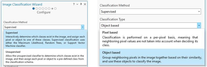
Figure 22.2 The Image Classification Wizard

For Classification Schema (Figure 22.3), if you have an existing set of informational classes that you wish to use, this would be the input for that dataset. If you do not have a set of informational classes, choose NLCD2011, the National Land Cover Dataset for North America, the default schema for ArcGIS^® Pro. Or your employer/organization may have one you must use when classifying imagery. This chapter will not demonstrate the Optional inputs of Segmented Image and Reference Dataset. Segmented Image is used with Object based classification with the Reference Dataset an already classified image. Training Samples will be used and discussed later in this chapter and more extensively in Chapter 23.

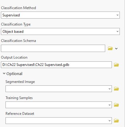
Figure 22.3 Developing a classification schema

Select Next to proceed to the Training Samples Manager of the Wizard. (Figure 22.4). Training samples are created by the analyst (you) by selecting pixels within the satellite image that represent specific spectral values that can be associated with informational categories. We will discuss the creation of the samples later in this chapter.

The next tab of the Wizard is called Train. This provides three options as the Classifier method—Random Trees, Support Vector Machine, and K-Nearest Neighbor. The descriptions are found in Figure 22.4 and are only three of the many possible supervised classification methods within the Image Classification Wizard.

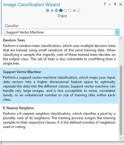
Figure 22.4 The Training Samples Manager  tool

The Image Classification Wizard walks you through the classification process step-by-step. Still, as noted in the prior chapter, the image generated is only useful within the map project where it was created. The most frequently used supervised classification method, maximum likelihood, is unavailable from the Image Classification Wizard. We will demonstrate the use of the wizard in Chapter 24: Conducting a Supervised Classification. 

Geoprocessing Tools

Geoprocessing tools provide additional options for classification. Under the Analysis tab, select Tools, and search first for “classification” (results on the left in Figure 22.5) and then search for “classify” (right in Figure 22.5). Many more results are available for classification. Not all of these are classification methods, which include Maximum Likelihood, Forest-based Classification, Regression Classify Pixels using Deep Learning, and Classify Objects using Deep Learning. Most of these methods are beyond the scope of this book. Each of these classification methods has its own support documentation section in the ArcGIS^® Pro (under Help). We encourage you to consult academic literature to better determine which approach best supports your project.

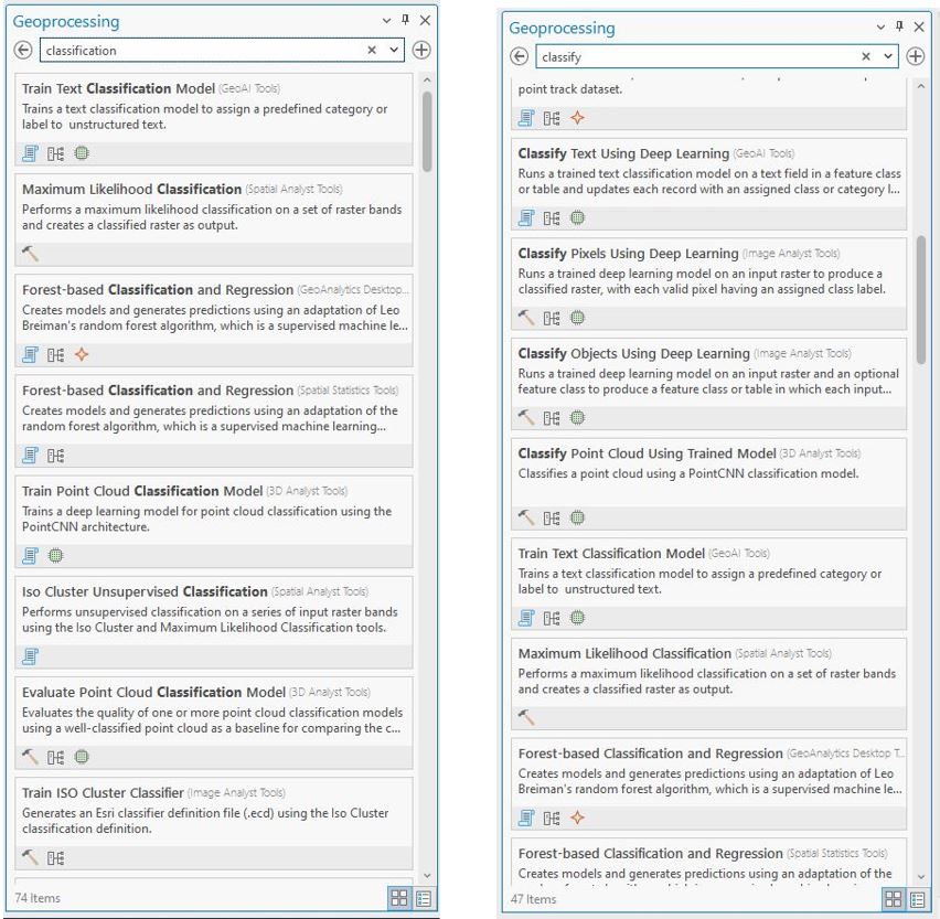
Figure 22.5 Classification options in the Geoprocessing tool

Within Chapter 24, we demonstrate the Maximum Likelihood and Classify Raster tools. These tools create a new image usable in other map projects. But using these tools requires more tools, including Train Maximum Likelihood Classifier (this chapter) and Create Signatures (Chapter 24)—processes that are directly incorporated into the Image Classification Wizard. We will demonstrate those tools independently of the Image Classification Wizard, as it is important to understand the basics of supervised classification.

Creating Training Samples

The first step associated with supervised classification is creating training samples, a sample of spectral values characterizing each informational class. The training sample file is then used in supervised classification to evaluate the spectral values of all pixels in an image and to assign them to a specific informational class.

Training samples can be created within the Image Classification Wizard by using a specific tool for the method, such as Train Maximum Likelihood or Train Random Tree Classifier. But another way is found under the Imagery tab Classification Tools, called Training Samples Manager (Figure 22.6).

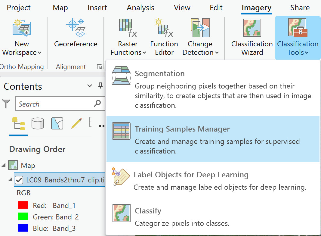
Figure 22.6 The Training Samples Manager tool

Since we will demonstrate three different processes in ArcGIS^® Pro, we want to create one training sample file for all three methods. We will use the Training Samples Manager.

Open the Training Samples Manager by clicking on the icon. An informational classification schema is already built into the Training Samples Manager—NLCD 2011¹. Figure 22.7 shows only the top part of the tool. We will show the rest as we proceed.

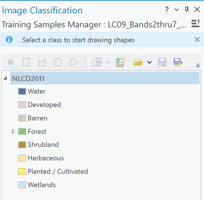
Figure 22.7 The NLCD 2011 classification schema

ArcGIS® Pro does not require that this informational class scheme be utilized. Select the Create New Schema icon (right in Figure 22.8) if a new one is desired. Or, if an informational class schema already exists that you need to use, click on the folder to navigate to that Classification Schema (left in Figure 22.8).

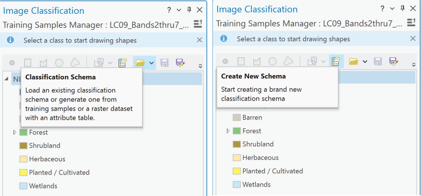
Figure 22.8 Accessing training sample schema tool options

Modifying an Existing Classification Schema

We can start with the NLCD 2011 and modify it as needed. This will be demonstrated in this chapter. Remember, we only need four informational classes.

Right-click on the name of any of the information classes listed under NLCD2011. In Figure 22.9, we right-clicked on Shrubland. As seen in the pop-up box, classes can be added, removed, or edited. Since we only use four informational classes, we must remove the others.

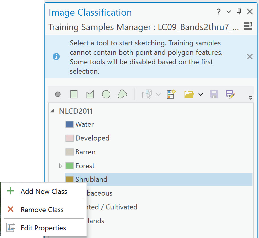
Figure 22.9 Removing a class

Select Shrubland, right-click, and select Remove Class. Don’t worry! As seen in Figure 22.10, ArcGIS^® Pro asks before it is removed. Select Yes.

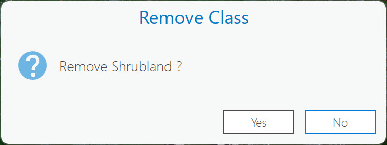
Figure 22.10 Removing a class

Remove other classes until only four remain – Developed, Planted/cultivated, Forest, and Water (Figure 22.11). If you accidentally removed too many, don’t worry; we will show you how to add a class back again.

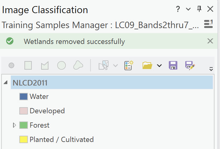
Figure 22.11 Removing a class

Once only four classes remain, rename them to correspond with the informational classes outlined below.

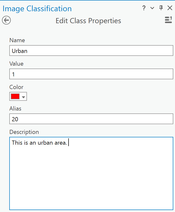
Figure 22.12 Changing the class properties

Please do the same for each of our informational classes (Figure 22.13).

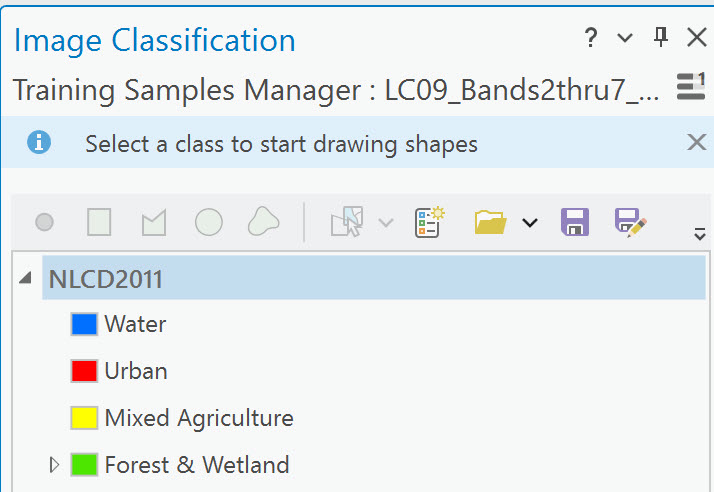
Figure 22.13 Changing information classes

Remember, we are working with these four informational classes only. If you removed an informational class by mistake, you could add a new class by selecting the green + button to add a new class and name it for the one accidentally deleted (Figure 22.14).

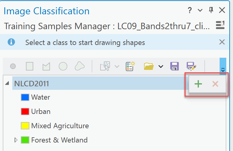
Figure 22.14 Adding an information class

Saving the Classification Schema

There are two ways to save the classification schema: Save or Save as. We will use Save As to save your classification schema as a new file. Otherwise, the NLCD2011 schema will be overwritten with our changes. Click Save As, name the new classification schema, and in Output Location, confirm that this file is saved in the correct folder (Figure 22.15).

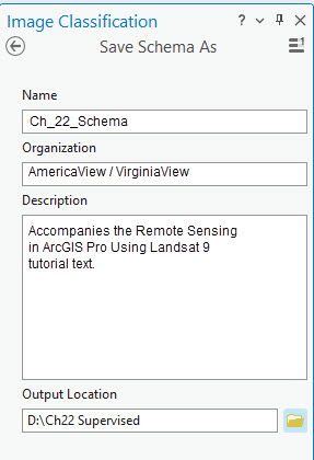
Figure 22.15 Saving the modified schema

Creating Training Samples

Now that the classification schema has been created, we will create training samples.

Go to the bottom half of the window (Figure 22.16). If a training sample already exists, it can be loaded by selecting the folder Load Training Samples.

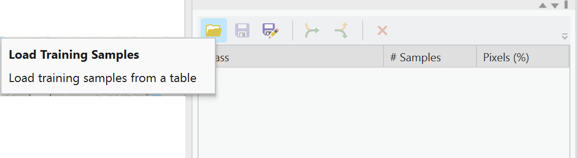
Figure 22.16 Loading training samples

 

Since we do not have any existing training samples to load, we will create our own using the drawing tools at the top of the window (Figure 22.17).

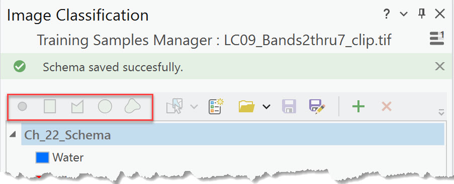
Figure 22.17 Creating training samples using the drawing tools

The drawing tools include Rectangle, Polygon, Circle, or Freehand. While creating training samples, you may need to switch between various band combinations in your image (Chapter 16) to help identify features.

Let’s start with water—Zoom in to Smith Mountain Lake in the southeast portion of the image (Figure 22.18).

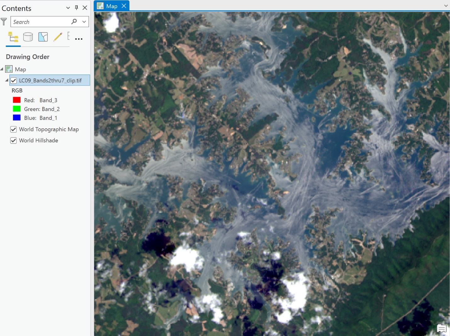
Figure 22.18 An image of Smith Mountain Lake

Select Water in the Image Classification tool and click Circle (Figure 22.19).

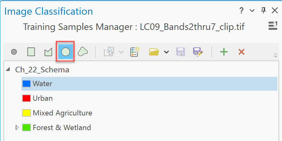
Figure 22.19 Creating training samples using the circle tool

Place the cursor, now crosshairs to indicate drawing, anywhere in the lake’s body. Be sure to stay away from shorelines; we don’t want to capture any of those as spectral values for water. Once an appropriate location is found, drag outward to create the circle. Figure 22.20

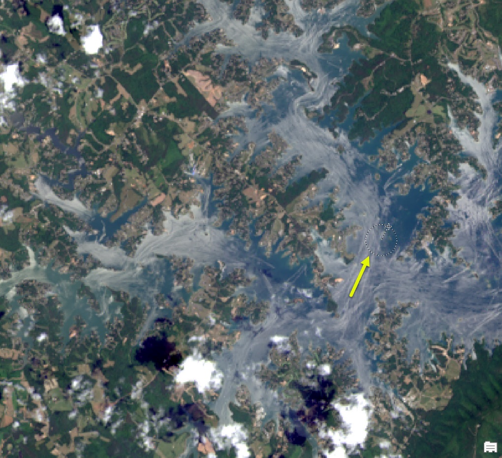
Figure 22.20 Creating training samples using the circle tool

Again, stay away from the shoreline, and capture only water pixels (Figure 22.21)

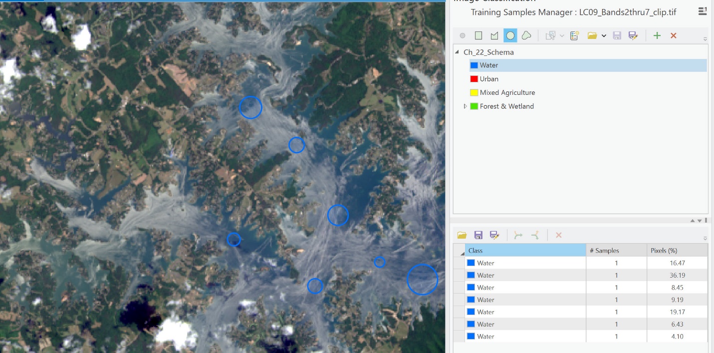
Figure 22.21 Creating training samples using the circle tool

If you don’t like the sample of pixels you captured (too many or too few), select the row for the Water sample and choose Delete. Figure 22.22. Don’t worry; sometimes, it takes a few tries to get the hang of selecting samples.

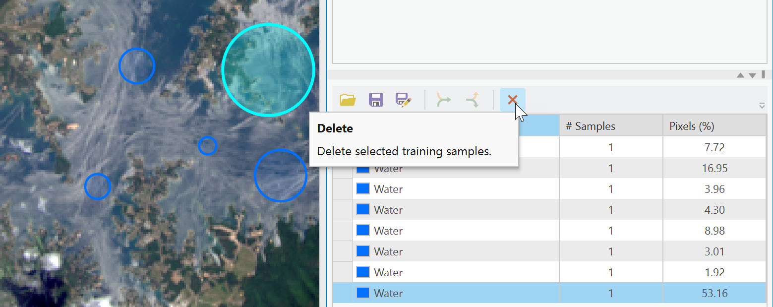
Figure 22.22 Creating training samples using the circle tool

Zoom in and out and navigate the scene to pick up additional water pixels for this lake. If you are uncomfortable with the Circle, the Polygon tool is most effective for non-symmetric areas. Note in the figure below that we also captured some of the water that is a bit turbulent. Remember, the point is to get samples of different spectral values related to a specific feature. Figures 22.23 and 22.24

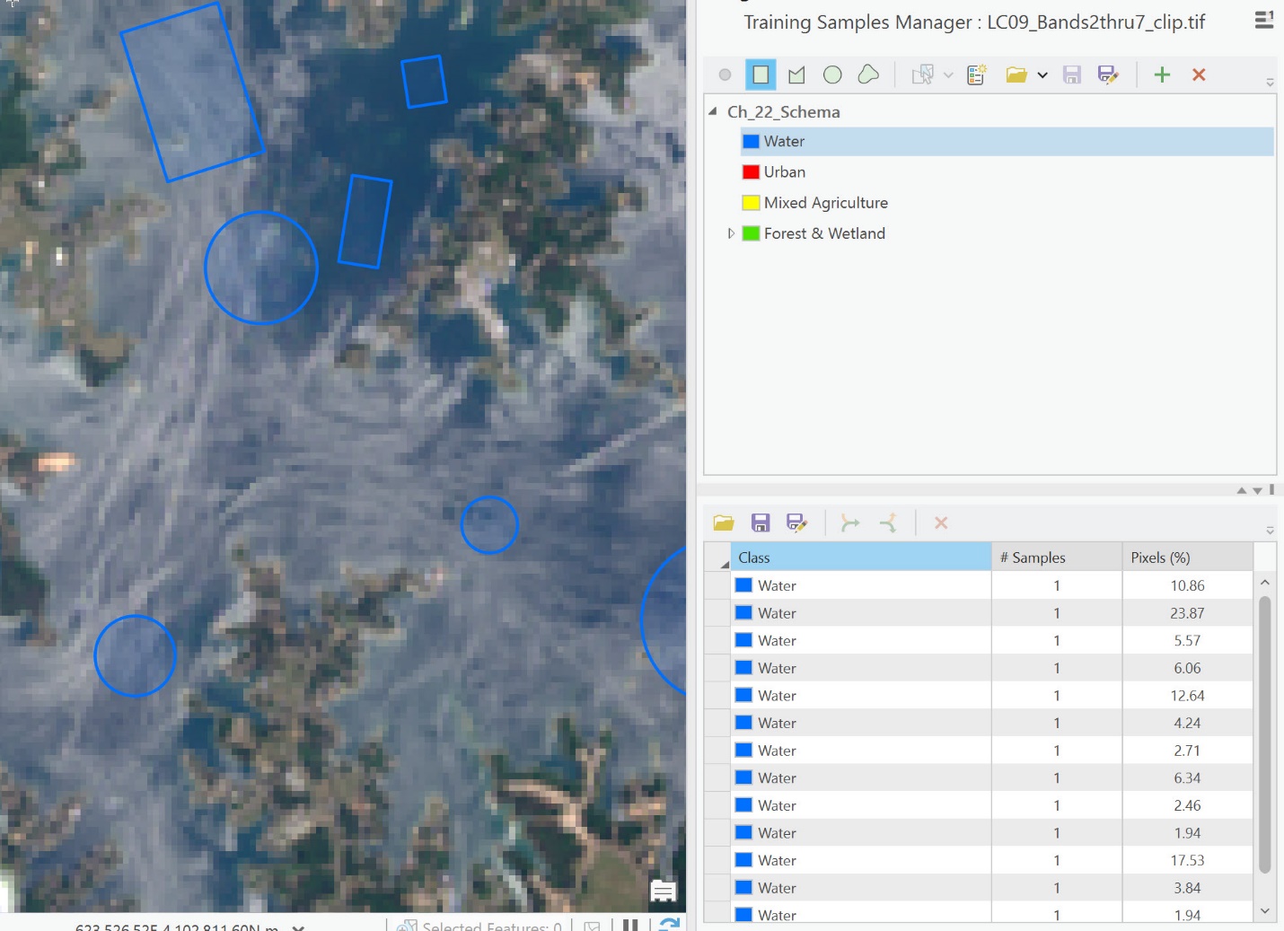
Figure 22.23 Creating training samples using the rectangle tool

Don’t forget the other water bodies in the image (Figure 22.24). If needed, you can change your band combinations to help you better locate water (Figure 22.24). As training samples are added to the map viewer, each is listed as a separate row in the Training Samples Manager.

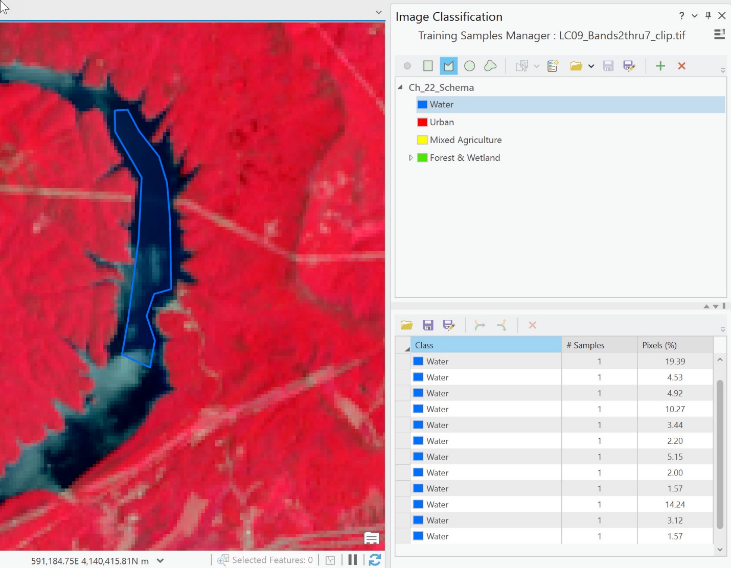
Figure 22.24 Creating training samples using the freehand tool

We recommend frequently saving your training samples (Figure 22.25). This is not the same file as the classification schema—this process will create a shapefile of the training samples. Name the training sample file so that you understand its purpose (Ch 22 training samples).

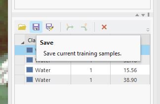
Figure 22.25. Saving training samples

Save frequently so that if ArcGIS^® Pro closes, the work will not be lost.

Once finished with water, move on to training urban, forest, and agriculture. Don’t forget to select the class name at the top of the Training Sample Manager dialog box before training the next class.

Figure 22.26 illustrates an urban training sample. As in Chapter 21: Unsupervised Classification, we are not concerned with individual features within an urban area. For this exercise, all streets, parks, golf courses, etc., within the urban area will be classified as urban.

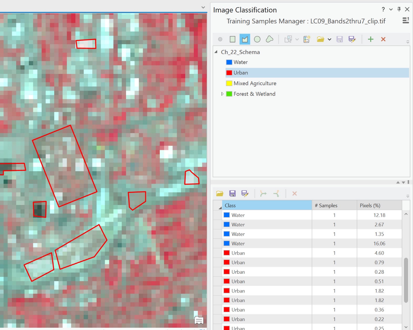
Figure 22.26 Selecting urban feature samples

When complete, the image in the map viewer will display all the training samples (Figure 22.27). Collect samples across the entire geographic spread of the image. Avoid collecting any one class from a single location or region. And be careful to avoid getting too close to the edges of water or including roads in forest and agriculture. In ArcGIS^® Pro, the training samples for an individual informational class are color-coded according to the color scheme at the top of the Training Sample Manager dialog box. For example, forest training samples are green, urban areas are red, agriculture fields are yellow, and water is blue. BE SURE TO SAVE!

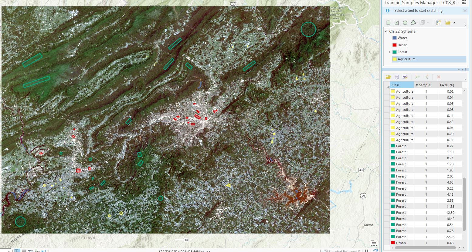
Figure 22.27 Viewing all training samples

When have you collected enough training samples? It depends on the area, the variation in spectral signatures of the land cover, and the project. Again, sample different regions of the image, different types of agriculture, forest, urban and water areas. In the next section, we evaluate the spectral coverage to determine if we have collected sufficient training samples.

Save both your training samples and your project. You may get the following message when trying to close your project (Figure 22.28). This is a warning message that not everything has been saved. So be sure to click Yes.

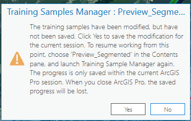
Figure 22.28 Saving training samples

Please proceed to the next chapter, which provides the step-by-step process to evaluate the training samples. Training samples must be evaluated (Chapter 23) before conducting the supervised classification (Chapter 24).