17 Chapter 17: Radiometric Enhancement of Landsat 9 Imagery

Overview

The next three chapters introduce image enhancement using ArcGIS^® Pro. This chapter demonstrates radiometric enhancement.

Image Enhancement: An Introduction

Image enhancement denotes processing of remotely sensed imagery to adjust brightness values represented as digital numbers (DN), thereby improving the image’s visual qualities for a specific purpose. The brightness values of individual pixels are changed to enhance qualities such as color balance, brightness, contrast between pixels, or other characteristics.

An image’s visual quality is connected to the range of pixel brightness values, known as contrast. An image with high contrast has a narrow range of brightness values – largely only blacks and whites. An image with low contrast has a wide range of brightness values, is often associated with black and white images, and includes gray pixels. Usually, extremely low contrast is undesirable, as features will appear not as blacks and whites but as intermediate greys. Often, these values may better record the important features of an image (than just black and white), but the gray tone may also suppress key features within the image. On the other hand, extreme reduction of contrast may conceal distinctive features within a scene.

Image enhancement permits the application of a level of contrast appropriate for a specific purpose. Of particular significance is the recognition that the intent of image enhancement is to improve an image’s appearance for that specific purpose. Because analyses have different objectives and images have differing qualities, preferred enhancement techniques vary from application to application. Image enhancement is a manipulation of an image’s appearance, so fundamentally, image enhancement is cosmetic and should not be used as an input for analytical purposes.

Most remotely sensed images require some form of image enhancement because images use only a small range of the brightness range available on a computer’s display. As such, many features in the image are not visible to the analyst. As a result, in its unenhanced form, the image’s suitability may be lacking for a specific purpose. Image enhancement expands the range of brightness used to display the image, thus revealing features not visible in the unenhanced version.

Enhancing images dynamically in a map viewer is much faster than creating a permanent image data file for every enhancement operation. Dynamic enhancement in a map viewer does not change the actual values of the pixels in the original image.

Histogram Enhancement Techniques

An image’s frequency histogram provides the best context for beginning an image enhancement discussion. A frequency histogram displays image brightness along the horizontal axis and the number of pixels at each brightness level along the vertical axis. The shape of a specific histogram is related to the features represented within a scene and the conditions under which the image was acquired. We provide examples of histogram enhancement techniques in this chapter. Some of these techniques are summarized below.

Linear Contrast Stretch expands the range of brightness values by extending the values to occupy the full range of brightness available within the image by creating new intermediate values.

Histogram Equalization expands the range of brightness by spreading the most frequent brightness along the brightness scale so that these values occupy the full range. The histogram of the enhanced image shows gaps between the brightness values because they have been separated to create a broader range of brightness in the image.

Digital Image Enhancement Techniques

A variety of digital image enhancement techniques are available. Choosing a particular technique depends on the application, data available, experience, and preferences of the analyst or the analyst’s customer. In this and the following two chapters, we demonstrate the three most important and widely used groups of enhancement techniques:

Radiometric Enhancement: Enhancing images based on the values of individual pixels (this chapter).

Spatial Enhancement: Enhancing images based on the values of individual and neighboring pixels (Chapter 18: Spatial Enhancement of Landsat 9 Imagery)

Spectral Enhancement: Enhancing images by transforming the values of each pixel on a multiband basis (Chapter 19: Spectral Enhancement of Landsat 9 Imagery).

Radiometric Enhancement using ArcGIS® Pro

We will use the first clipped 6-Band Composite Image created in Chapter 15: Sub-setting a Landsat 9 Image, the image clipped to the extent of the display. While we will continue to use the 6-band composite image (bands 2 through 7) in this chapter, enhancement techniques can also be accomplished on a single-band image.

To begin, create a new map project, name it, connect it to the project’s folder, and set the workspaces as demonstrated in previous chapters. Add the 6-band composite image.

Display the image in Color Infrared, band combination 4-3-2 ¹ (Figure 17.1).

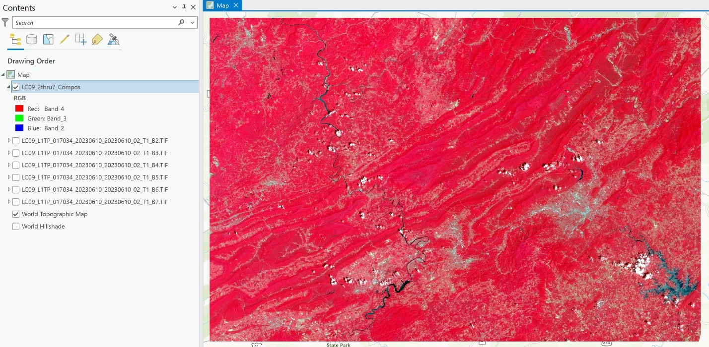Figure 17.1. Composite image

Select the Raster Layer tab on the ribbon.

We start with the Enhancement icons shown in Figure 17.2—Brightness, Contrast, and Gamma. These values may differ per user as the software sets the default values.

Figure 17.2. Brightness, contrast and gamma

The name of the enhancement tool can be viewed by pointing to its icon. Point to the sun icon (Figure 17.3). The tooltip indicates it is the Layer Brightness Enhancement tool.

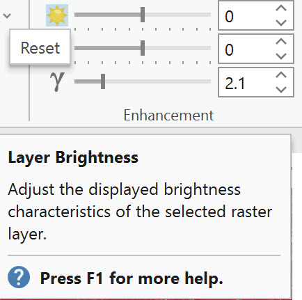
Figure 17.3. Layer Brightness

These three enhancement tools are adjusted using the slider, the up/down arrows in the box, or by typing a numeric value. Note: Once the values are changed, the image can be reset to ArcGIS Pro’s default values (which are 0, 0, and 1 respectfully). If you want to reset a modified value to a previous value, then you need to remember the what the initial values are prior to making a change (in this case [see Figure 17.3], 0, 0, 2.1). Click the icon corresponding to the setting you wish to reset (Figure 17.4).

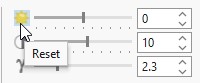
Figure 17.4. Reset

We will experiment with changing each value and observe the changes reflected in the display. Each enhancement technique changes the image display in different ways. Again, these techniques only change the display, not the pixel values in the original image.

Adjusting Image Brightness

Layer Brightness will make the image appear lighter or darker. The default value is 0; the value can range from negative to positive. Change the value as illustrated in the following two figures.

Negative values will darken the image. In Figure 17.5, the value was set to -30 (negative 30).

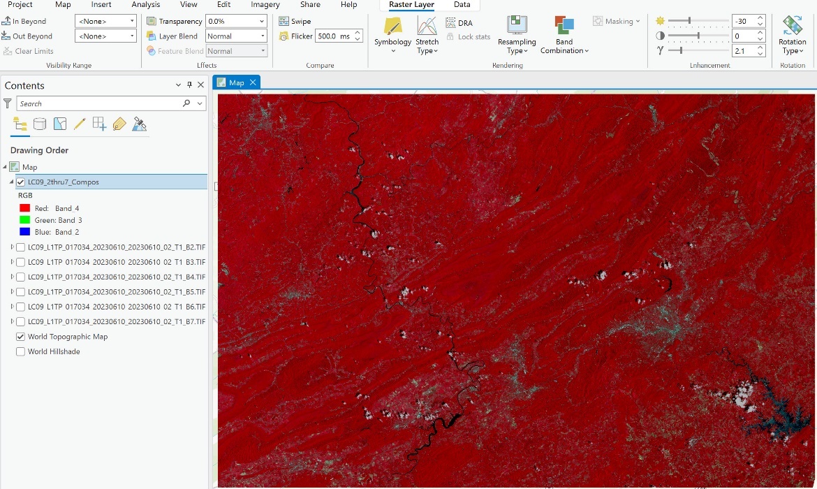
Figure 17.5. Adjusting image brightness

Positive values brighten the image. In Figure 17.6, the value was set to +14.

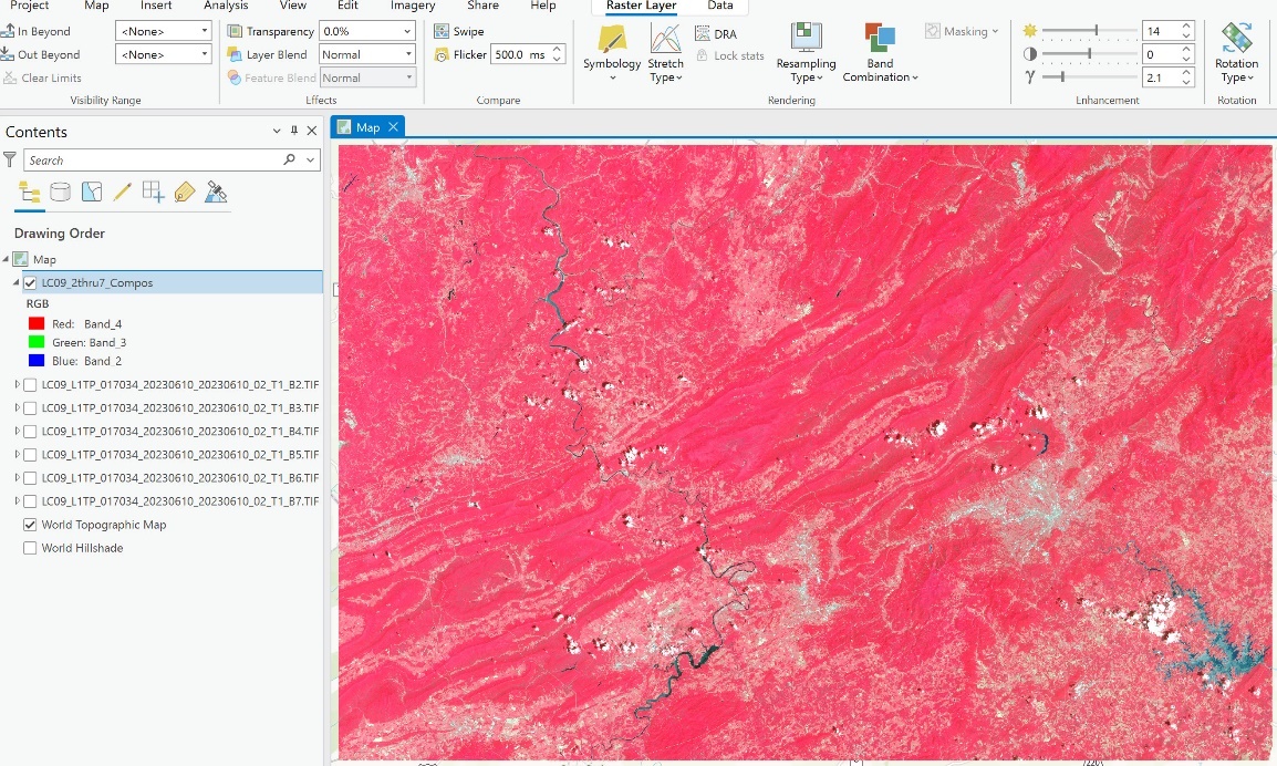
Figure 17.6. Adjusting image brightness

As demonstrated in the above two examples, brightening or darkening the image changes the individual features differently. The most appropriate enhancement technique is contingent on the specific project’s requirements. Change the brightness values to several different settings to see how the image changes.

When ready to move on to a different image enhancement technique, click the sun icon to reset the image to its default values before proceeding to Layer Contrast.

Adjusting Image Contrast

Layer Contrast changes the range of differences between the darkest and lightest objects. The Layer Contrast value in the figure below is set to 10 (Figure 17.7), and the slider bar is not centered. ArcGIS^® Pro automatically sets the Layer Contrast based on the image’s pixel values. When using a different image, the software might display a different value.

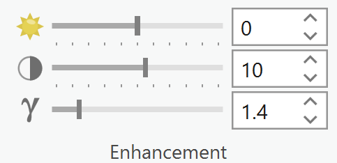
Figure 17.7. Layer contrast

Layer Contrast also has an adjustment range that includes negative numbers. Let’s try two settings.

In Figure 17.8, the contrast value was set to -35.

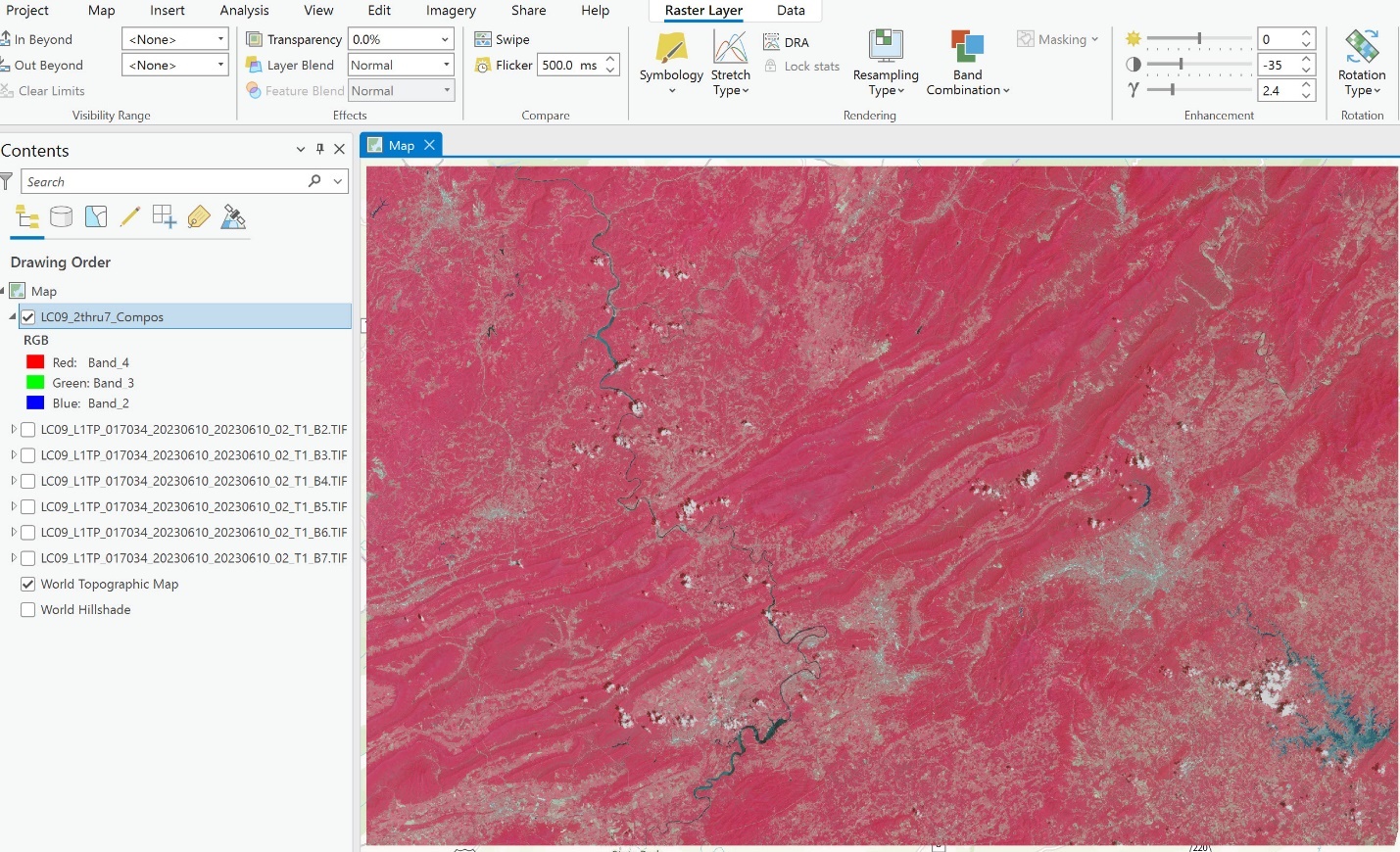
Figure 17.8. Muted layer contrast

Notice that the image appears to be darker, but it is actually not as sharp. The contrast is muted.

Now, increase the contrast value to +35, and a much sharper image displays (Figure 17.9). This setting has sharpened the difference between land and water bodies, which are the darker colored features.

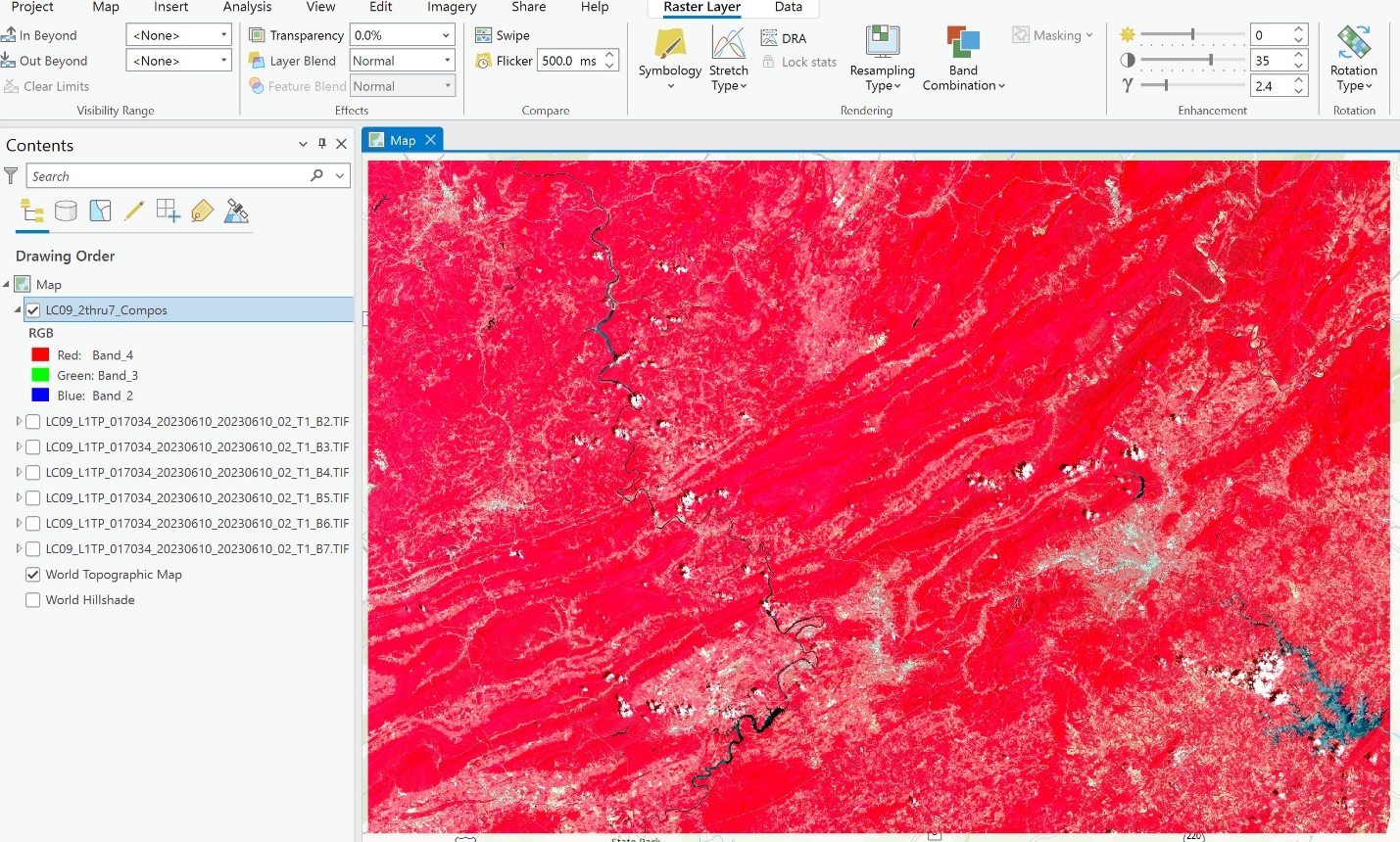
Figure 17.9. Exploring with layer contrast

Go ahead and try other settings. Remember to reset the values to default when finished. For Layer Contrast, the value resets to 0.

Gamma Enhancement

Layer Gamma controls the relationship between the brightness of the original scene and that on the display. For example, at a gamma of 1.0, the two images will use the same brightness scale. Whereas at a gamma of 0.5 or 1.5, the display shows either compressed or expanded brightness rankings relative to the original. For our image, ArcGIS^® Pro determined that 2.1 was the best setting (Figure 17.10). Layer Gamma values range from 0 to 10.0.

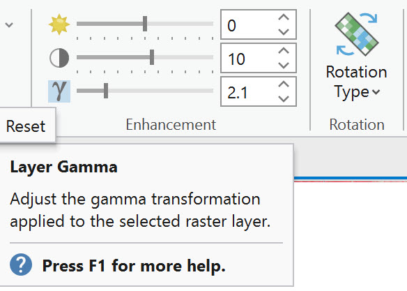
Figure 17.10. Gamma enhancement

In Figure 17.11, the Gamma value was set to 0.1.

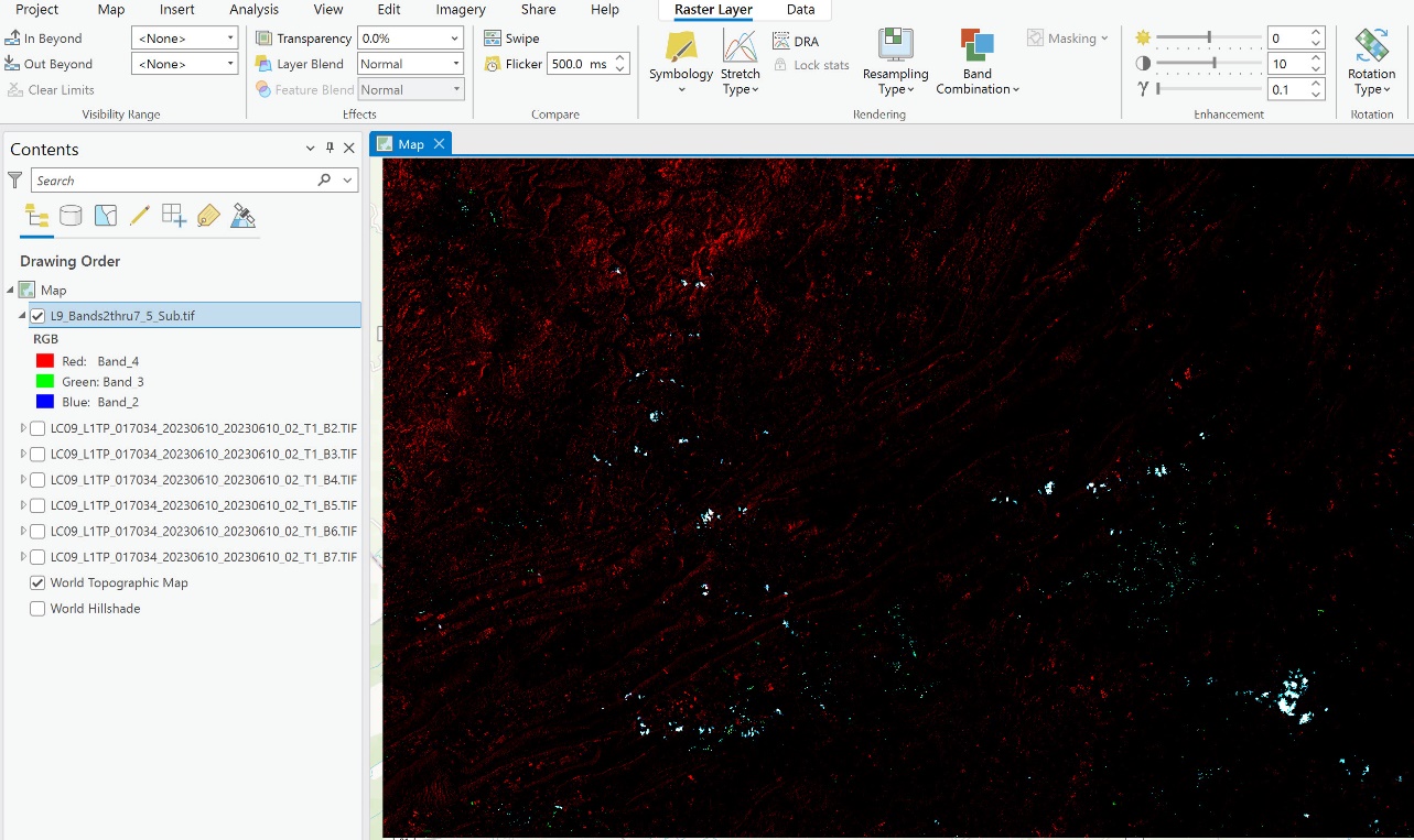
Figure 17.11. Setting a low Gamma value

In Figure 17.12, the Gamma value was set to 10.

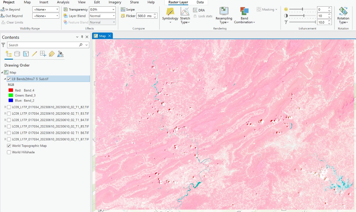
Figure 17.12. Setting a high Gamma value

What is the purpose of the two settings demonstrated? For this image, possibly nothing. But again, image enhancement settings are directly contingent on the application demands and the project’s goal.

Now reset the Gamma value to its default setting used by ArcGIS^® Pro.

Now, let’s look at another tool.

Dynamic Range Adjustment (DRA)

The Dynamic range adjustment tool (Figure 17.13) adjusts an image dynamically in the viewer when zooming in and out. The stretch type does not change; only the range of values changes based on the portion of the image (also known as the area of interest, or AOI) displayed in the viewer. This technique is used to help enhance a specific region seen within the viewer. The contrast stretch occurs seamlessly as the user pans around or zooms in or out of the image.

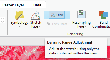
Figure 17.13. Enabling dynamic range adjustment

Figure 17.14 illustrates an example without DRA enabled.

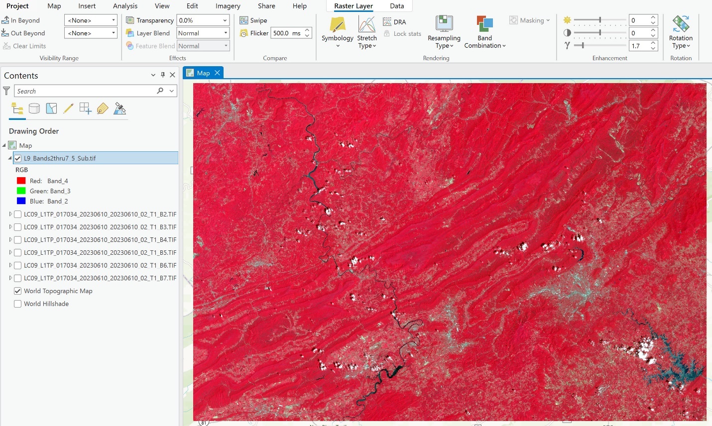
Figure 17.14 Image without DRA Enabled

Figure 17.15 shows the same image, zoomed in to view the crescent-shaped lake Carvin’s Cove without DRA enabled.

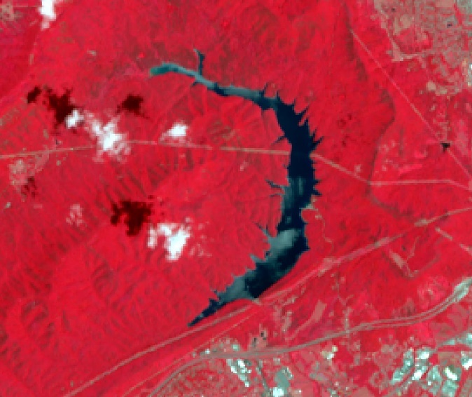
Figure 17.15. Carvin’s Cove without DRA enabled

Figure 17.16 provides an example of a DRA-enabled view of an entire scene. Visually, this figure is no different from a full image without DRA enabled.

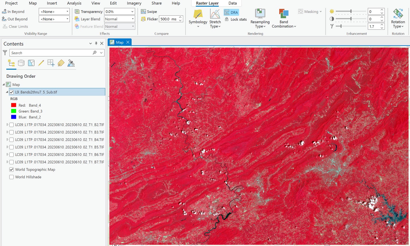
Figure 17.16. Full image with DRA enabled

The difference in the image display occurs when zooming in. Zoom in to Carvin’s Cove (Figure 17.17) with DRA enabled. The image is much sharper, especially the boundaries of the water body.

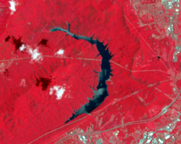
Figure 17.17. Carvin’s Cove with DRA enabled

Not sure if you see a difference? Turn off DRA. Zoom into the area in the black box in Figure 17.18 of the city of Roanoke.

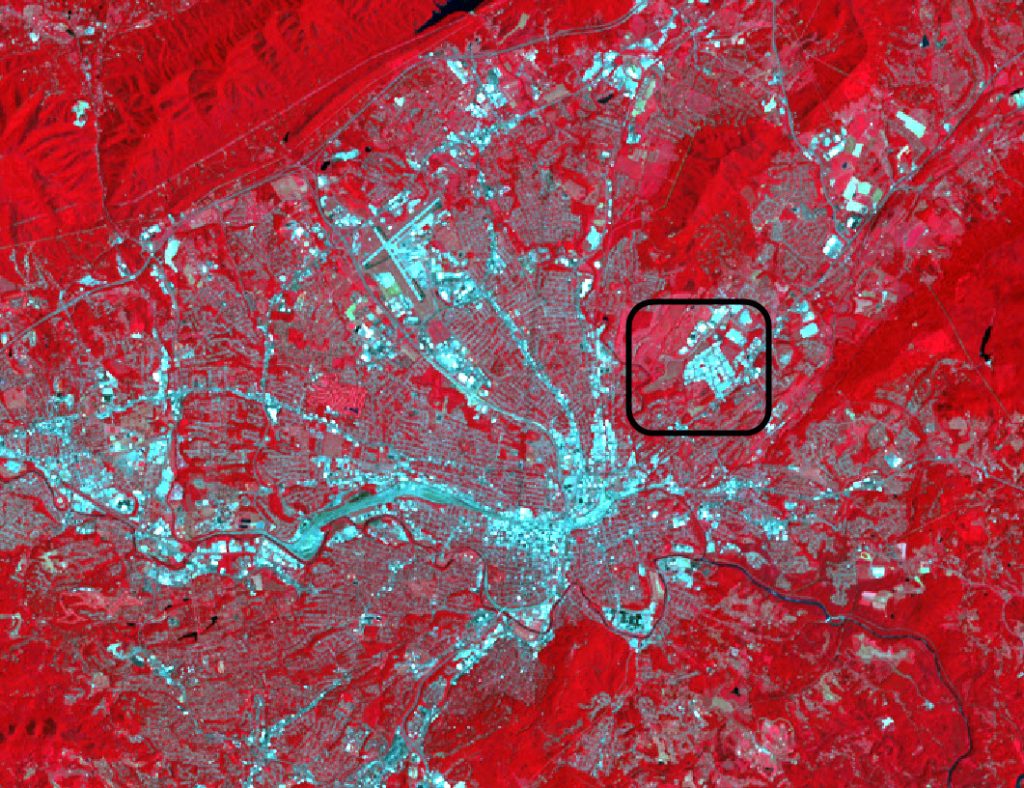
Figure 17.18. Area of interest of the City of Roanoke

Figure 17.19 shows the zoomed-in area without DRA.

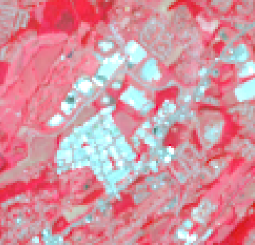
Figure 17.19. Zoomed-in area without DRA enabled

In Figure 17.20, DRA of the same area is enabled. The outlines of the buildings are much clearer than without DRA.

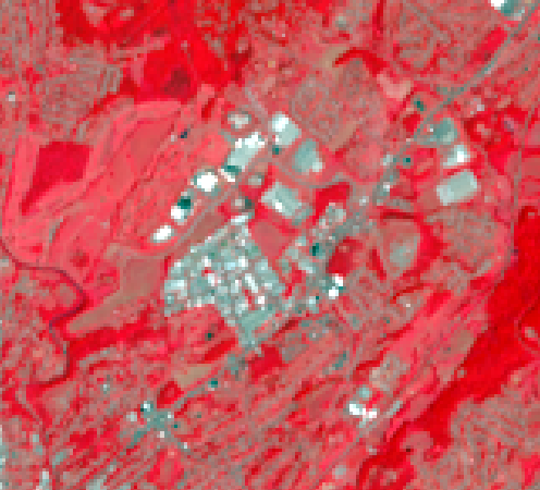
Figure 17.20. Zoomed-in area with DRA enabled

These tools are helpful when conducting image classification (covered in subsequent chapters) to help discern features within the image.

Set your image enhancement tools (Gamma, Contrast, Brightness) and DRA back to their original values before proceeding with the next section.

Histograms

As stated in the introduction, histograms plot the frequencies of brightness values, with the digital numbers (DN) along the x-axis and the number of pixels associated with each value on the y-axis. The shape of a histogram is determined by the features represented in the image and their brightness values.

Changing the Stretch Type changes the histogram and the image’s appearance in the map viewer. Go to the Raster Layer tab. Select the Stretch Type drop-down menu (Figure 17.21).

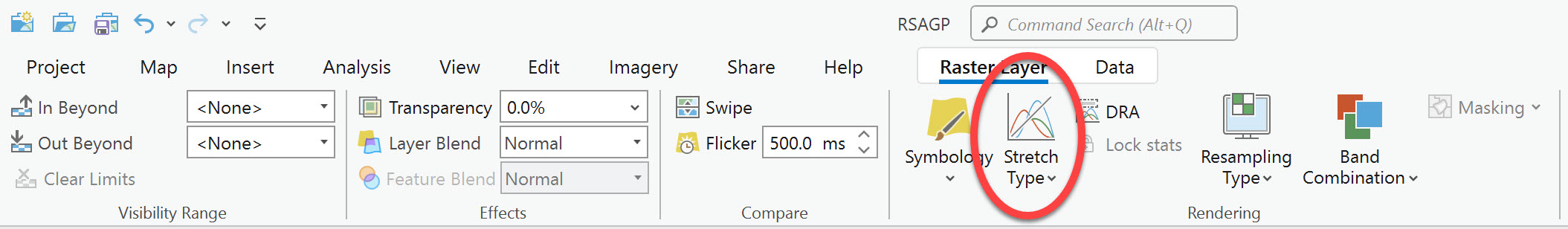
Figure 17.21. Changing the Stretch Type

A list of Stretch Types is provided (Figure 17.22). While defining these techniques below, we will only demonstrate enhancement methods used regularly. A complete review is beyond the course of this book, and academic literature should be consulted as to the best method for your project.

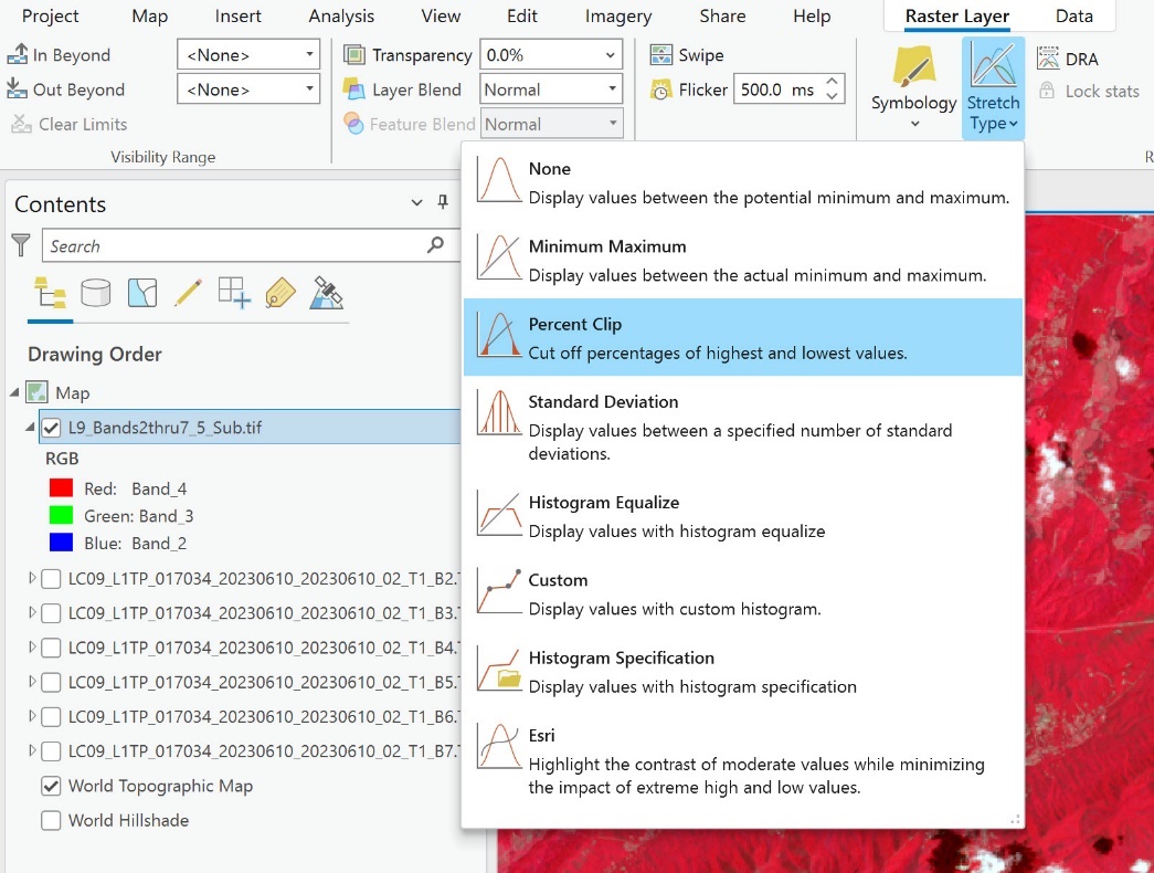
Figure 17.22. Percent Clip

 None displays all potential values.  The number of values will depend upon the sensor payload onboard the respective Landsat satellite (for example – Landsat 7 supports 256 values (8 bit), Landsat 8 is 12 bit resized to 16 bit, and supports 65,536 values; Landsat 9 is 14 bit and supports 16,384 values). You cannot manually adjust these values.

• Minimum–Maximum displays values between the actual minimum and maximum values in the image or values that you can independently set.
• Percent Clip is highlighted because it is the default. Percent Clip eliminates a histogram’s minimum and maximum value ends based on a percent. These values can also be changed.
• Standard Deviations displays values between a chosen number of standard deviations.
• Histogram Equalize reassigns the digital values to equally distribute them across the range of brightness values for the image. You cannot manually adjust the values.
• Custom is a manual specification, piecewise.
• Histogram Specification allows you to adjust the values using an uploaded .xml file.
• ESRI is the software-defined Histogram. You cannot manually adjust the values.

Let’s start by looking at the Percent Clip options. Go to Symbology and scroll down until Stretch type is visible, and if not already shown, change to Percent Clip by clicking on the down arrow at the end of the Stretch type line (Figure 17.23).

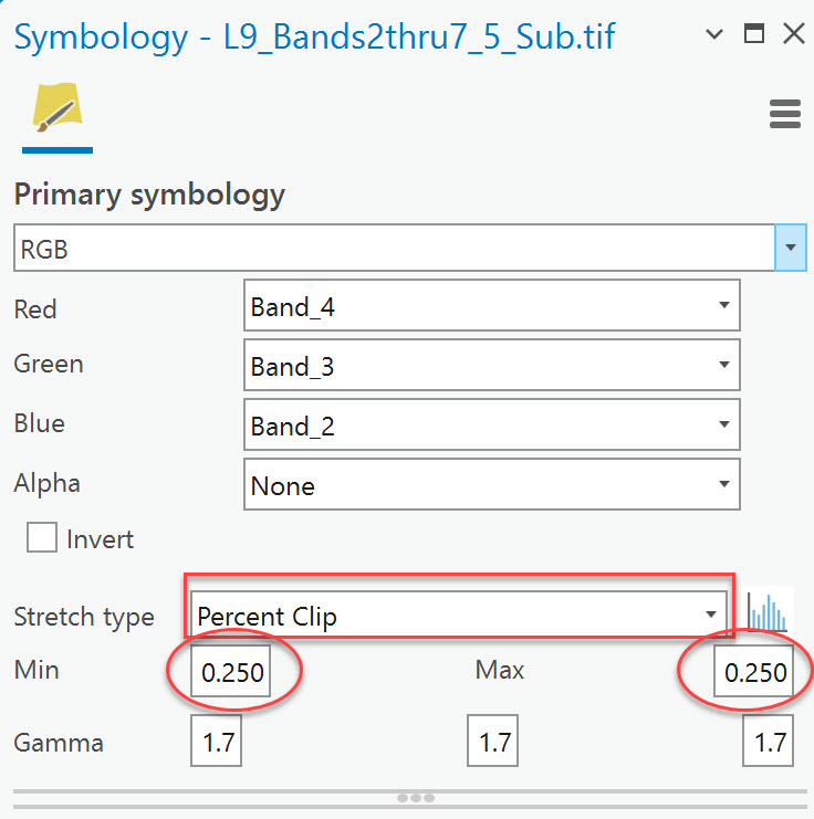
Figure 17.23. Percent clip parameters

Here it shows that the minimum and maximum ends of the Histogram were clipped by 0.250 (Figure 17.23). These values can be changed. Change it to 5.0 for both ends. The map viewer shows a substantial change, especially around the urban areas (Figure 17.24). The Statistics have not changed from the original setting because Statistics are based on the dataset values (remember this is dynamic enhancement).

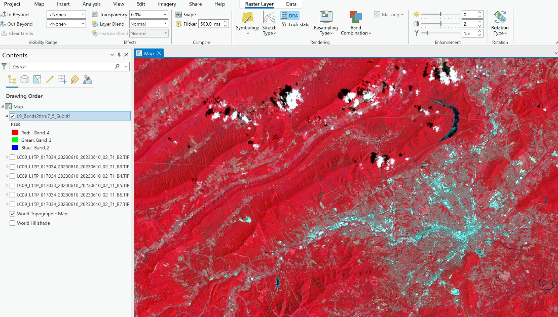
Figure 17.24. Map viewer after setting the percent clip

To change that, click the dropdown box next to Statistics under the Statistics tab (Figure 17.25).

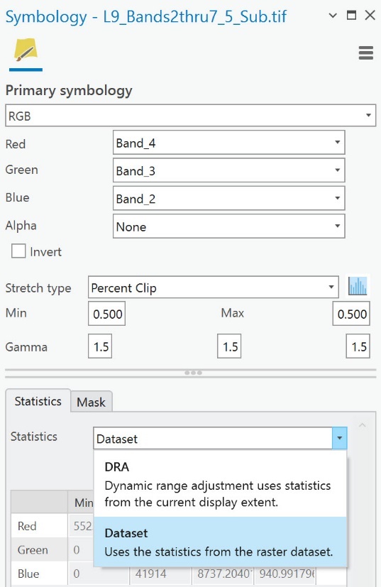
Figure 17.25. Changing the statistics parameters

Here the basis of Statistics can be changed. To set custom statistics, you must select a Stretch type other than Percent Clip and ESRI; we noted above that the values cannot be manually changed.

Change the Stretch type to see how this modification changes the image. Change to Minimum Maximum. How has the image and Symbology window changed? In Figure 17.25, the Minimum and Maximum Percent boxes are gone. The Statistics are still the same because they are based on the original brightness values in the image.

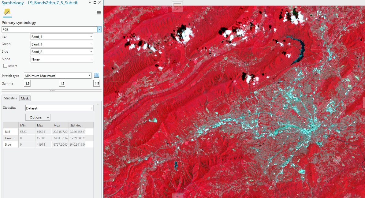
Figure 17.26. The image display

At the end of the Statistics line, select Custom (Figure 17.27).

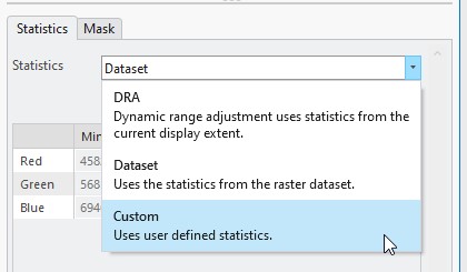
Figure 17.27. Selecting custom

You can change the numbers for each band by clicking in the box for the statistic and inputting the desired value. Remember that a 16-bit image has values from 0 to 65,535. In this image, the NIR band (displayed in red) has values ranging from 5,523 through 65,535 (Figure 17.28). Your values may differ depending on your selected area of interest (the area that you clipped).

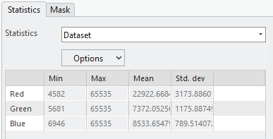
Figure 17.28. Band statistics

In Figure 17.29, we adjusted the minimum values to 0, and the maximum values to 65535

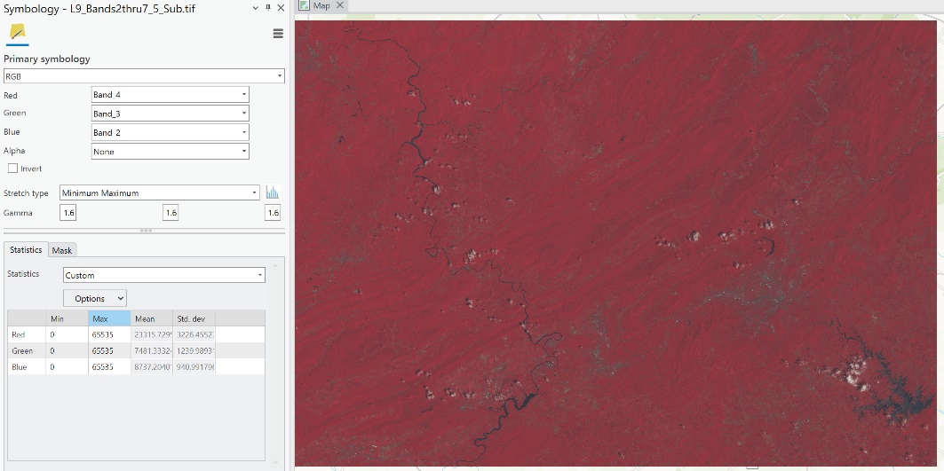
Figure 17.29. Image display

As you can see from this demonstration, the appearance of the image changed, but the brightness was not enhanced. So, when changing the statistics, should these be changed to 0 and 65,535 for a 16-bit image? The answer for this image is no. Should you for another image? That discussion is beyond the scope of this chapter because the range of values for any single band is contingent on the project for which the image is being analyzed.

You can reset the statistics by changing it back to Dataset.

The DRA setting will calculate statistics based on the extent in the map viewer. Zoom into the city of Roanoke, then select DRA from the Statistics drop-down menu. The statistics are not listed, but the image has changed to reflect the range of values in the extent of the image in the viewer (Figure 17.30). DRA demonstrated here is dynamically changing the appearance of the image using the DRA tool discussed above.

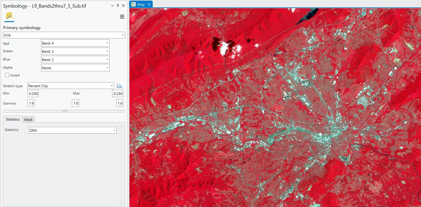
Figure 17.30. Image with DRA

Notice that Gamma is also present. All the settings for different forms of radiometric enhancement can be changed. These options do not need to be changed independently of each other. So, after adjusting Stretch type settings for any stretch type, Brightness, Contrast, and Gamma can also be adjusted.

Explore the various methods of histogram stretch with different band combinations. Which method is best will depend on the purpose of the project and likely a decision the analyst makes during the image analysis process. The goal of this chapter, and subsequent chapters, is to summarize the methods and techniques available in ArcGIS® Pro and not advise on which techniques to use.

Density Slicing

A final radiometric enhancement method is density slicing. However, density slicing is not an available option on a composite image. Density slicing can only be performed on each individual band image in ArcGIS^® Pro. Density slicing differs from contrast stretch in that it assigns colors to specific brightness values. The colors do not add information but permit the analyst to make sharper distinctions between brightness classes in the image. This technique is beyond the scope of this chapter. However, the process is performed using the Spatial Analyst tool called Slice. 

Viewing and Exporting a Histogram

To view the histogram associated with a specific band, select the composite image raster layer in Contents and go to the Data tab on the ribbon. Select Create Chart – Histogram (Figure 17.31).

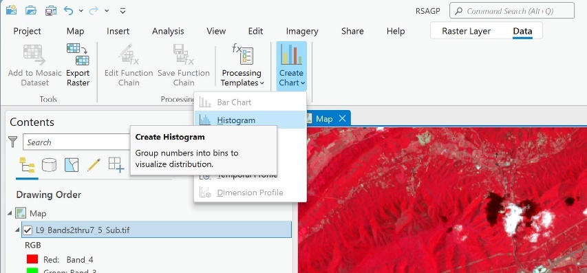
Figure 17.31. Creating a histogram

An empty histogram chart and the Chart Properties pane open under the map viewer (Figure 17.32).

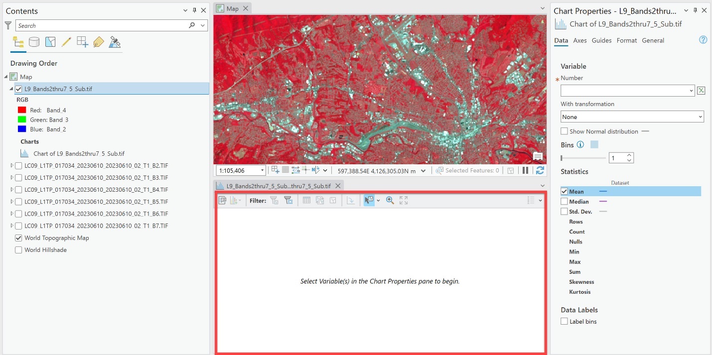
Figure 17.32. Charting

Using the drop-down box under Number, select a band. The only bands available are those currently displayed, bands 4-3-2 in this example (Figure 17.33).

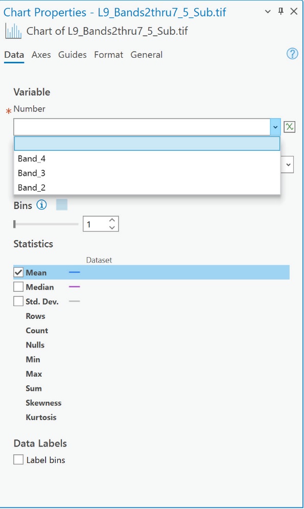
Figure 17.33. Chart properties

Choose Band_4. When a Band number is selected, the histogram appears in the Chart window. The blue line on the Histogram is the mean line – because Mean is the only Statistic checked in the Chart Properties window (Figure 17.34).

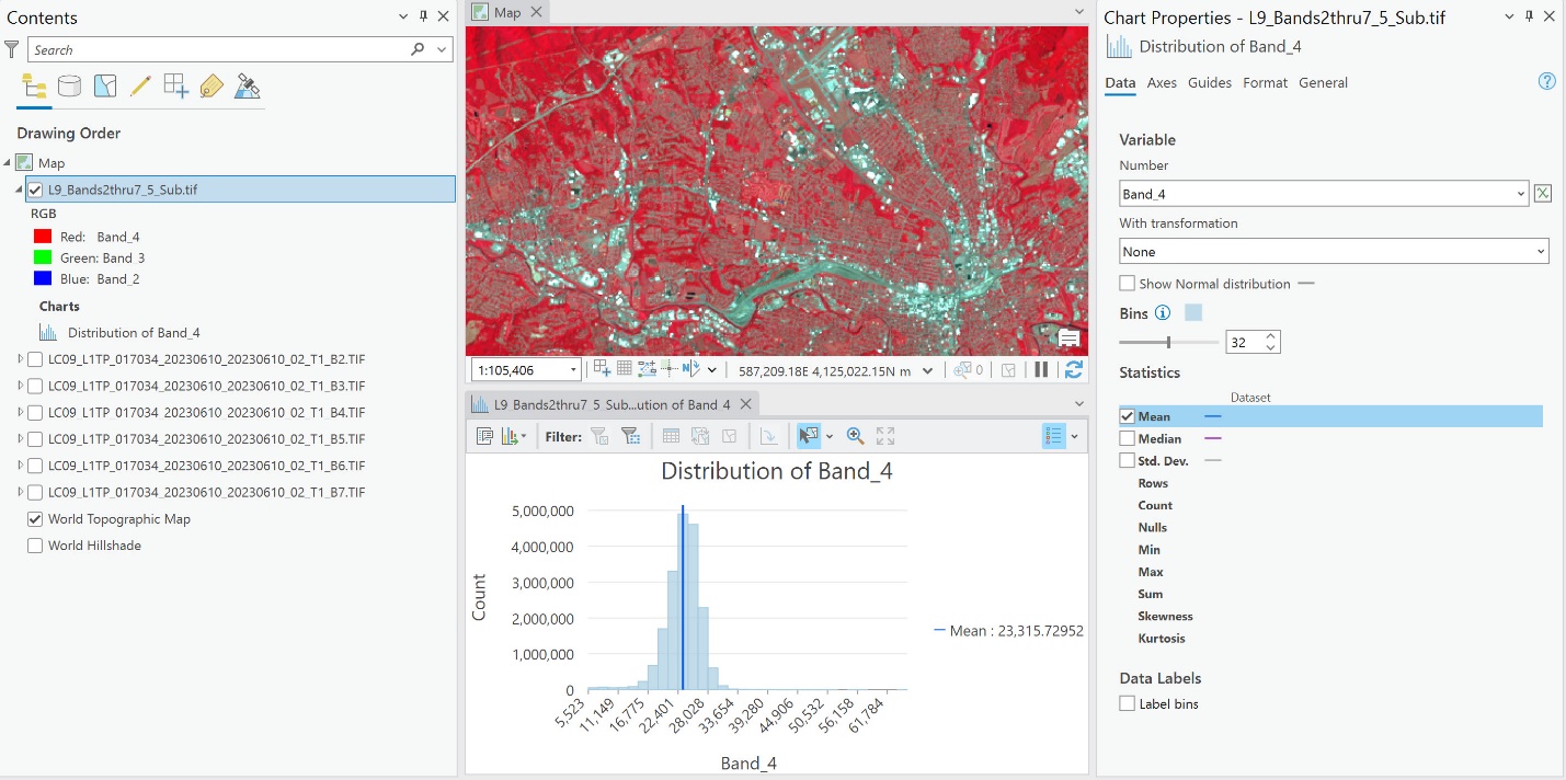
Figure 17.34. The chart properties window

Choose the other two statistics—Median and Standard Deviation (Figure 17.35).

Books

Figure 17.35. Median and standard deviation

The Axes and Format tabs at the top of the Chart Properties pane can be used to change the formatting of the histogram. We will not review these.

The General tab provides additional options to display on the Histogram (Figure 17.36).

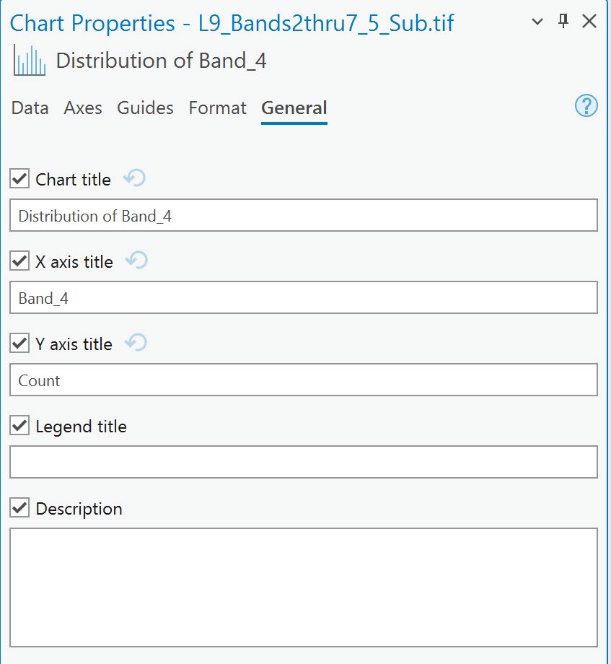
Figure 17.36. Additional histogram display options

Now change the Band number to Band_3 (Figure 17.37).

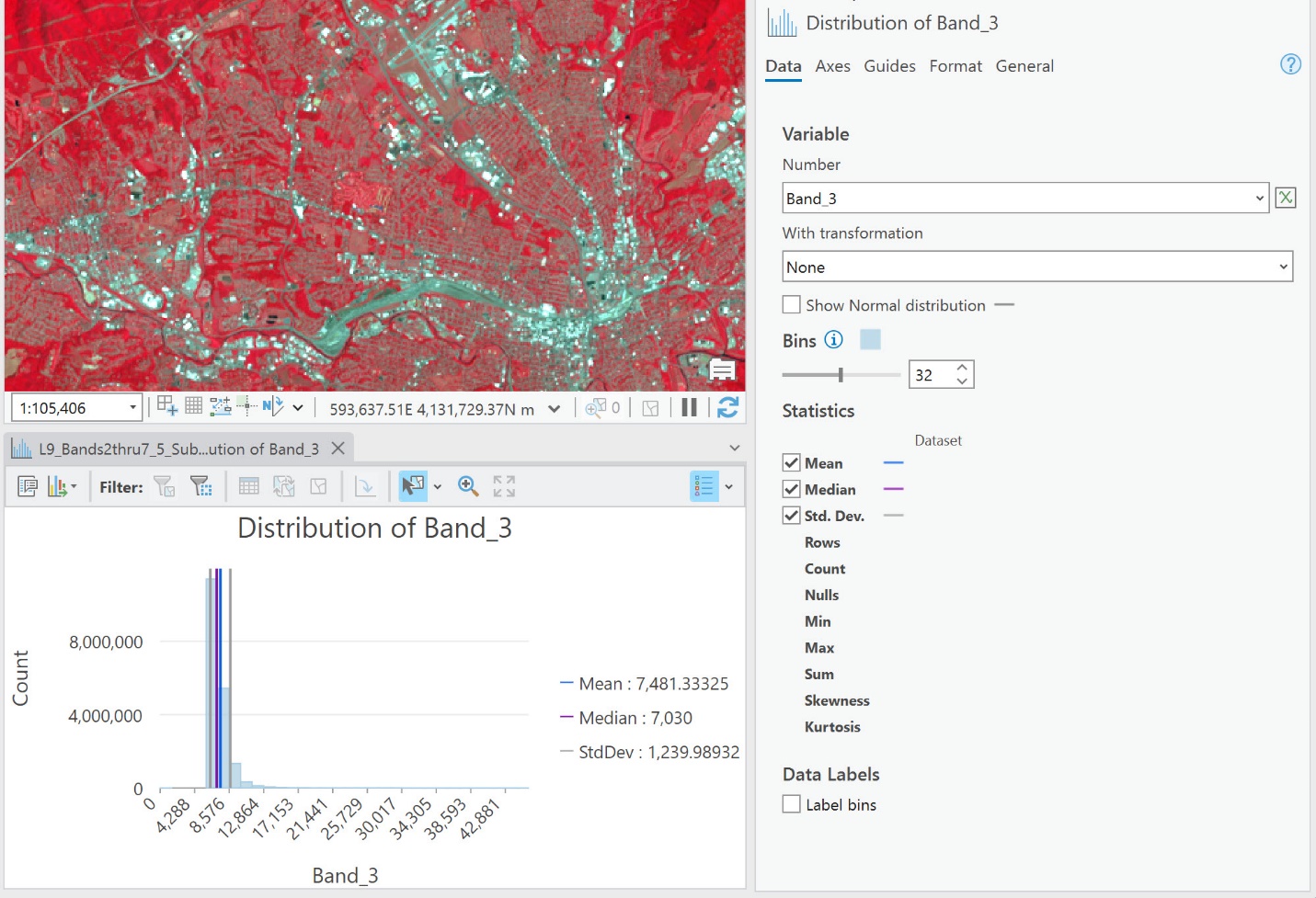
Figure 17.37. Changing bands

The histogram associated with Band 3 looks very different from Band 4’s histogram. Recall the discussion about Band Combinations from Chapter 16? Chapter 16 also provided an overview of the spectral properties of features on the Earth’s surface. Remember that each feature on the Earth’s surface reflects, absorbs, and re-emits different types and values of electromagnetic radiation in different ways. These features often have unique spectral signatures. The variation in histograms between the different Landsat Bands demonstrates these spectral variations.

If a histogram is needed for a figure in a non-GIS format, click on Export in the Chart window.

This ends the chapter on radiometric image enhancement. We will discuss further image enhancement techniques in the following two chapters. Spatial enhancement enhances images based on the values of individual and neighboring pixels. We cover spatial enhancement in Chapter 18. Spectral enhancement transforms the values of each pixel on a multiband basis, such as Band Ratios or Vegetation Indices. We cover spectral enhancement in Chapter 19.