14 Chapter 14: Creating a Composite Image using Landsat 9

Introduction

Landsat images are acquired in grayscale, so when added to ArcGIS^® Pro, each image, or band, is listed separately in the Contents pane. Familiarity with a Landsat scene is essential to complete analyses such as change detection, unsupervised classification, supervised classification and to generate other indices such as NDVI. Image processing and image analysis techniques are covered in subsequent chapters.

Creating a composite image means creating one image from several different bands. Landsat images can be displayed in natural color or red-green-blue (RGB) with a composite image. Displaying multiple bands in color allows features within a scene to be distinguished from each other. This helps differentiate between land cover types, including urban areas, forests, agriculture, and water bodies, for example.

Recall from discussions in prior chapters that data contained in each band comprises a different slice of the electromagnetic spectrum. Wavelengths can vary in the number of bands and wavelength ranges between Landsat sensors and from one satellite system to another (for example, Landsat and Sentinel). Figure 14.1 provides the wavelengths covered by Landsat 9 sensors.

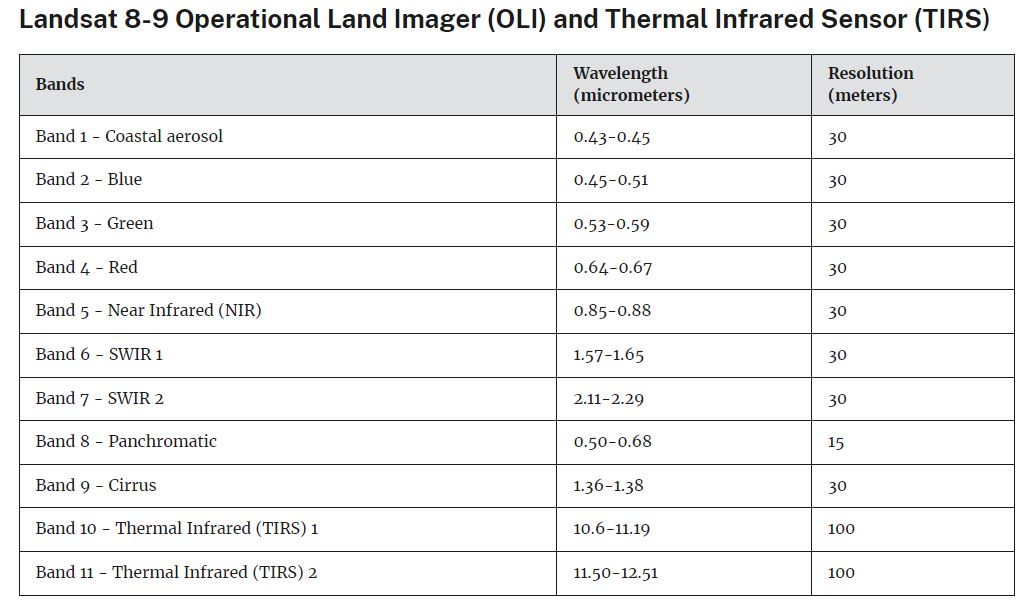
Figure 14.1 Spatial and spectral resolution of Landsat 8 and 9. Source: USGS (https://www.usgs.gov/faqs/what-are-band-designations-landsat-satellites)

We will generate two different composite images for this exercise using two methods. Compositing an image means combining more than one spectral band into a single image.

Before beginning this Chapter, be sure to complete Chapters 12 and 13. Open the project created in Chapter 13. Ensure your project has layers in descending numerical order in the Contents pane and all symbology is grayscale, as seen in Figure 14.2. We recommend that you turn off any base map.

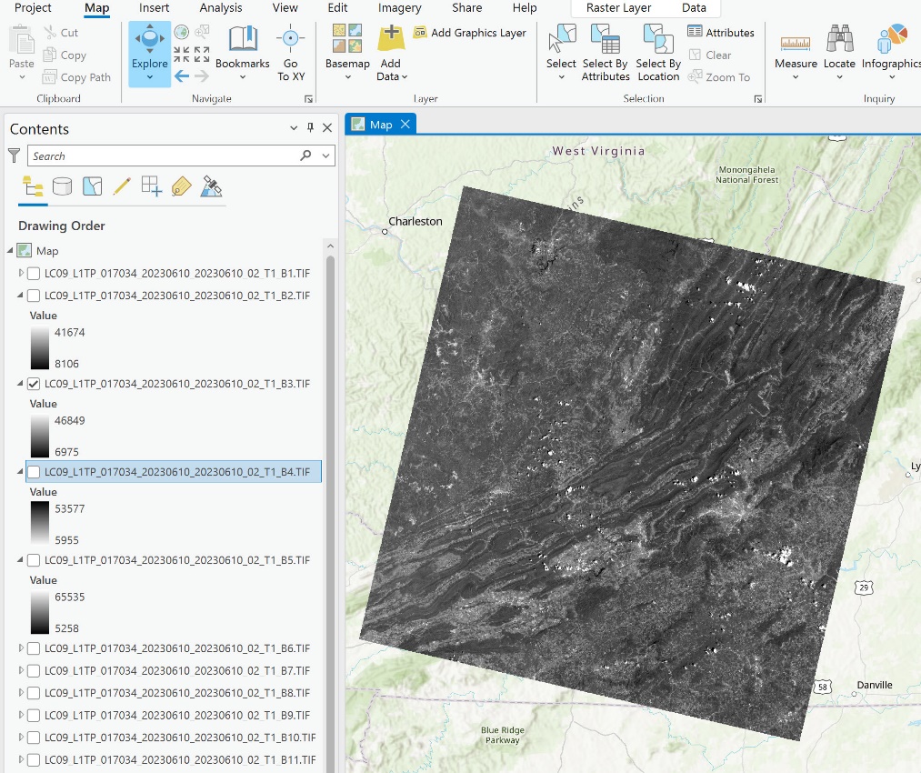
Figure 14.2. Landsat image in the map display

Next, check the workspace environments by going to the Analysis tab on the ribbon and select Environments from the Geoprocessing group (Figure 14.3).

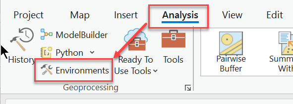
Figure 14.3. Selecting Environments

Ensure the Current Workspace and Scratch Workspace (Figure 14.4) are set to the project’s geodatabase. If not, use the browse option at the end of the input box to navigate and connect to the geodatabase.

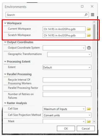
Figure 14.4. Setting the correct workspace

Now we are ready to create a composite image. We will demonstrate compositing using a geoprocessing tool and an imagery process shortcut tool, and we will use all eleven bands of the Landsat imagery for both examples. 

Creating a Composite Image using Geoprocessing Tools

You can find the Composite tool under the Analysis tab. Select Tools from the Geoprocessing group (Figure 14.5). Tools opens the Geoprocessing pane, providing a shortcut to Geoprocessing capabilities.

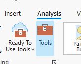
Figure 14.5. Tools

In the Geoprocessing pane, search for Composite and select Composite Bands (Data Management Tools) from the results (Figure 14.6).

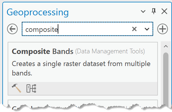
Figure 14.6. Search for composite in Tools

In the Composite Bands tool, the Input Rasters consist of the individual bands, and the Output Raster will be the name of the newly created composited image (Figure 14.7).

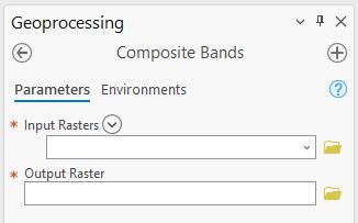
Figure 14.7. The Composite Bands tool

Choose the down arrow for Input Rasters and select the Band 1 image from the list, which will populate the box. A line is added to enter the next band. Continue this process until all eleven bands are entered, ensuring the bands appear in descending numerical order in the tool list, as shown in Figure 14.8. This importance will become apparent when the composite image has been generated.

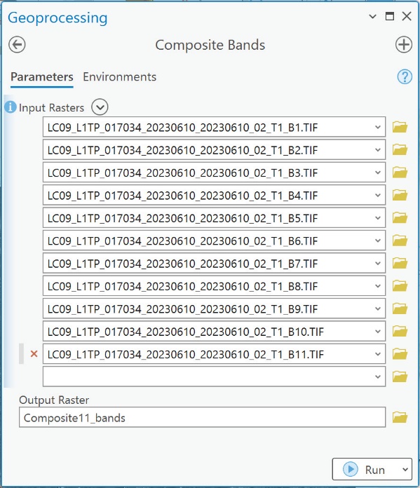
Figure 14.8. Entering bands in sequential order

Under Output Raster, name the new raster. For ease in remembering what this new raster represents, we have named it Composite11Bands. We recommend including the band numbers in your naming convention, so you know immediately which bands were used.

When typing the name, ensure it is saved into the project geodatabase (.gdb).

Once everything is populated, click on Run at the bottom of the tool.

Be patient; each of these eleven bands represents a large file individually, and they will all be combined to form one (huge) composite multispectral image. The processing progress is shown at the bottom of the tool (Figure 14.9).

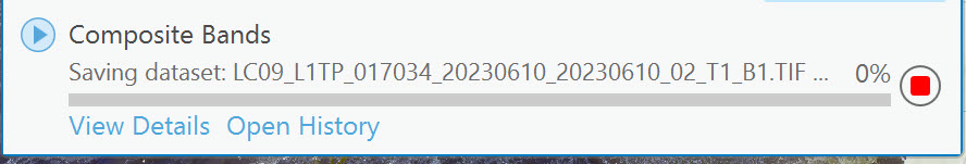
Figure 14.9. Processing an 11-band composite image

Once finished, the processing status box will turn green (Figure 14.10).

Figure 14.10. Processing complete

If a red message states that the processing failed, try the tool again, ensuring the output raster is saved in the geodatabase.

Once the tool has completed, the Contents and map have a new layer – a composite (multispectral) image created by combining the 11 separate bands (Figure 14.11).

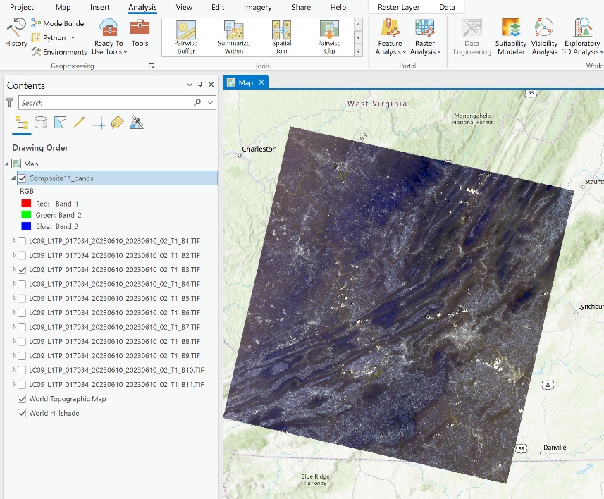
Figure 14.11. A composite multispectral image

The composite image in Contents displays the default symbology—Red, Green, and Blue. The image in the map window appears to be in color. ArcGIS® Pro displayed Band 1 in Red, Band 2 in Green, and Band 3 in Blue. Notice that although the image is in color, the color does not appear natural. It looks slightly blue, and the colors and contrast seem somewhat muted.

From the table in Figure 14.1, Landsat 9, Band 2 is the blue visible range of the electromagnetic spectrum. Band 3 is the green visible, and Band 4 is the red visible. Because the colors displayed by ArcGIS® Pro do not align with the band colors in the Landsat image, natural colors are not displayed. We can change the symbology and show different bands with either red, green, or blue color combinations. This process will be covered in Chapter 16: Band Combinations using Landsat 9 Imagery.

Only three bands are displayed, so did the composite for eleven bands work? Right-click the layer and choose Properties and Source from the menu in the left pane. Expand the Raster Information category. (Figure 14.12). This shows it is an eleven-band image.

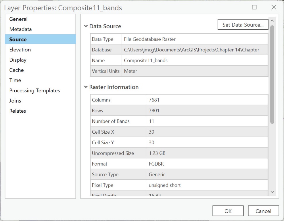
Figure 14.12. Information about the composite image

Which band is which band? This is why ensuring the bands were in order was necessary. When we change symbology (see Chapter 16), the bands must be inputted in the correct numerical order (Figure 14.13).

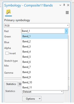
Figure 14.13. The composite band sequence

Save your project!

Making an Image Composite using the Imagery Process Shortcut Tool

This section demonstrates the same process using the shortcut tool.

Select all the individual band layers in the Contents pane, but do not include the composite image created in the last section. Select the Imagery tab (Figure 14.14) on the ribbon, then select the Process menu (Figure 14.15). Multiple options are available here—Clip, Mask, Difference, Composite, and Mosaic. Select Composite; the other options will be discussed in later chapters.

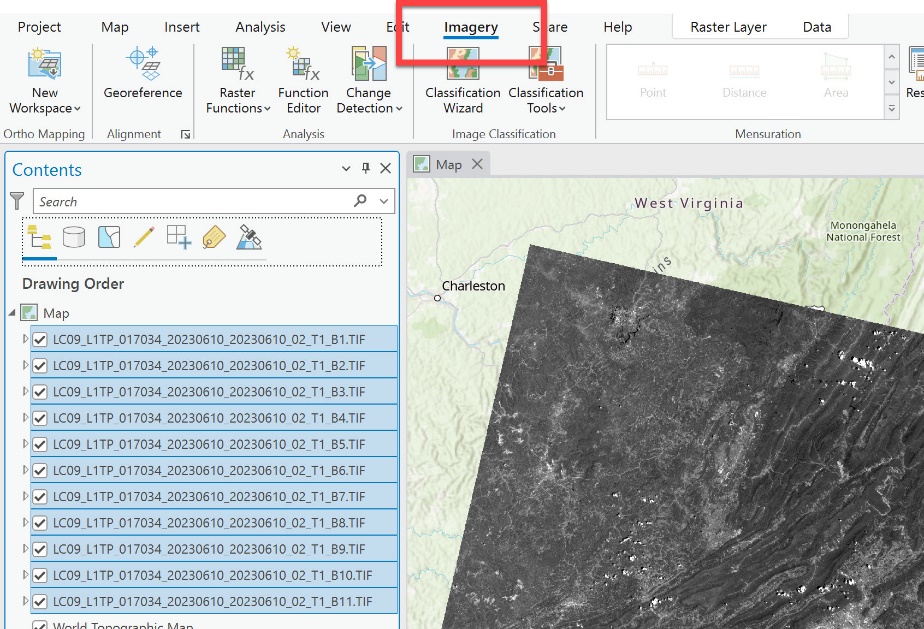
Figure 14.14. Accessing the Imagery tab

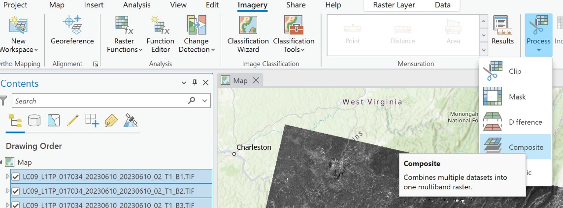
Figure 14.15. Selecting the Composite option

Choose Composite, and the processing automatically occurs with a new layer called Composite in Contents (Figure 14.16). Be sure to save your project as soon as the new image appears.

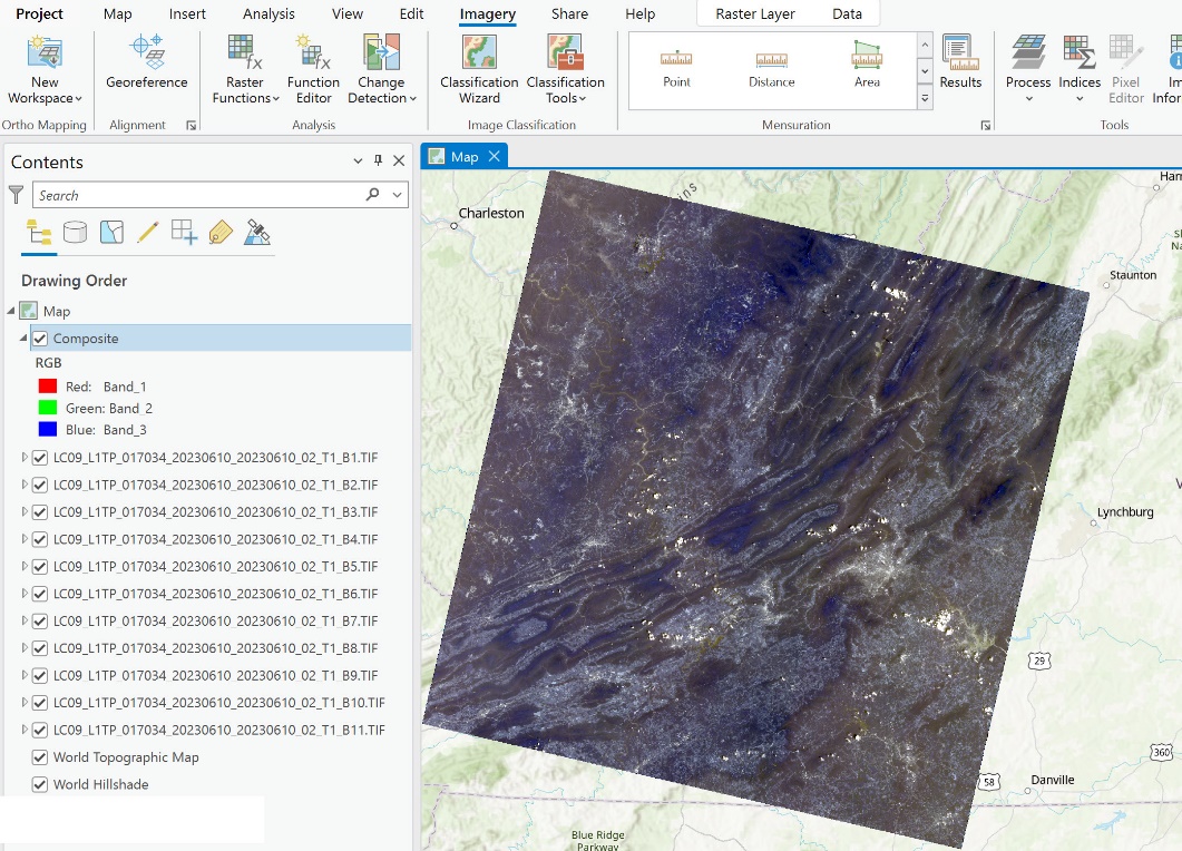
Figure 14.16. Generating an image composite

From this process, it is apparent from Contents that a new composite image with the default name Composite has been created and added at the top. Three bands are displayed—Red, Green, and Blue. Are the other bands present after this process? Check the Properties/Source/Raster Information for the image; it is an eleven-band image (Figure 14.17).

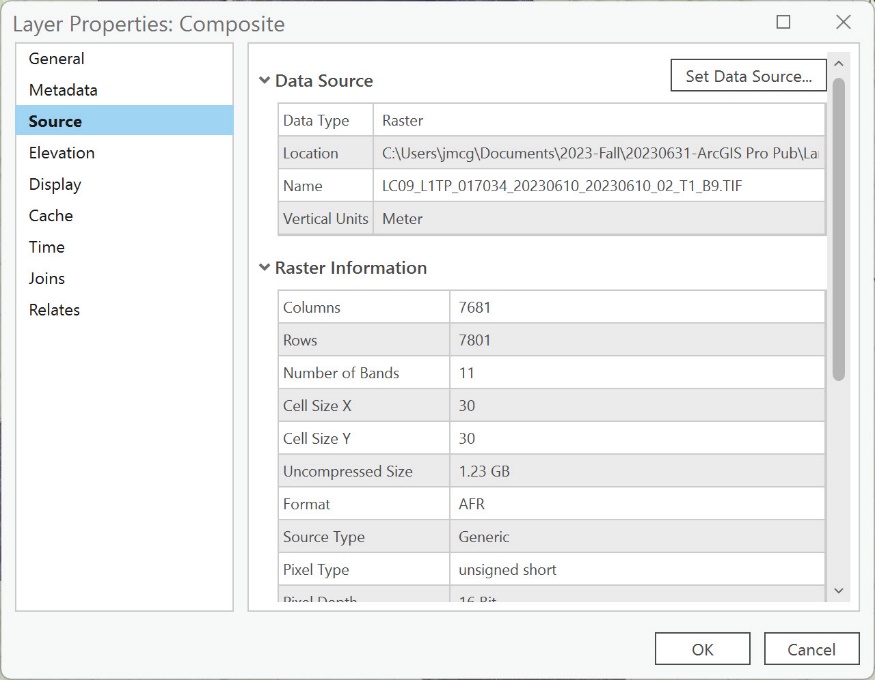
Figure 14.17. Accessing information about the new composite image

The symbology for this image shows that Band 1 is displayed as Red, Band 2 as Green, and Band 3 as Blue, just as the image created from the Composite Bands Geoprocessing tool. Similarly, notice that the new image’s color, like the Composite11Bands image, also does not appear natural—it looks slightly blue. The two composite processes appear to produce the same result.

Conclusions

We demonstrated how to create a composite image using the geoprocessing and shortcuts tools. Which process is better?

The composite image created using the shortcut tool is not a permanent image that can be used in other analyses and is only present in this project. If you check your workspace in Catalog, the file is not shown, nor does it appear in the geodatabase; if you closed the project without saving (or ArcGIS® Pro closed for any reason), the file would no longer be available. Why use the shortcut tools? Perhaps the only thing needed was to inspect the Landsat imagery for different band combinations and display, not an analysis.

Is using all eleven bands of a Landsat 9 scene necessary when creating a composite image? No, a composite image can be accomplished using any selection of bands. We recommend that you only include the specific bands required for the project when creating a composite image. However, be careful when generating a composite image; ArcGIS® Pro renumbers the bands. If all the bands are not used, or one band in a sequence is eliminated, the band numbers in ArcGIS® Pro will not correspond with the individual spectral band numbers for the Landsat image. For example, if Bands 2 – 5 are the only bands used (blue visible through near-infrared), once composited, the band numbers will be represented in ArcGIS^® Pro as bands 1 – 4. In this case, carefully document and note the specific bands used.

But what if, during the Geoprocessing operation, you failed to note which bands were used? How do you verify which bands were used and, if used, in which order?

ArcGIS^® Pro documents your processing steps. Go to the Analysis tab, and click History (Figure 14.18).

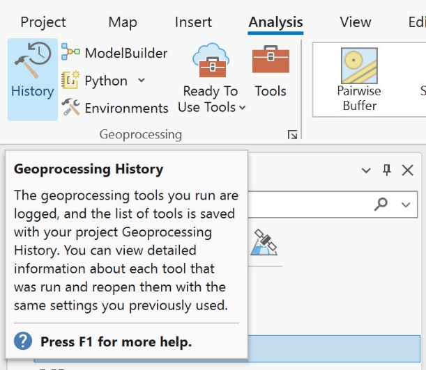
Figure 14.18. Accessing history

In the History pane (Figure 14.19), point to Composite Bands, and a pop-up displays the input order. The pop-up is not very reader-friendly, which is why documentation is essential when completing processing.

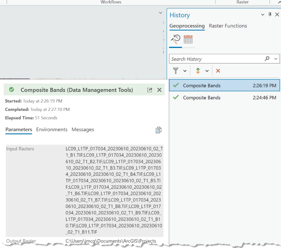
Figure 14.19. Processing history

Why do we bother creating a composite image? The human eye can only see that portion of the electromagnetic spectrum within the visual range. By creating a composite image, we can display, using the RGB color scheme, different bands that not only include data from the visible spectrum, but we can also substitute bands from outside the visible spectrum to expand the scope of the regions of the spectrum our image can represent. This allows us to view images of features we cannot normally see.

Integrating imagery from outside the visible spectrum is a powerful analysis tool. For example, thermal data can support emergency management applications such as identifying hot spots when fighting wildfires. Image analysis incorporating the near-infrared spectrum is often used to identify stress in agricultural crops long before the stress is evident to the human eye, providing agricultural operators with the ability to not only prevent crop loss but also to maximize production while minimizing inputs such as fertilizer, herbicides, pesticides, and water.

Save and close your project and proceed to Chapter 15: Subsetting a Composite Landsat 9 Image.