13 Chapter 13: Displaying Landsat 9 Imagery in ArcGIS® Pro
Introduction
The Landsat 9 scene downloaded in the previous chapter provided eleven different images, each with a different band designation and each covering a specific region of the electromagnetic spectrum. In this chapter, we will add the eleven individual bands (TIF files) to ArcGIS® Pro and examine the properties of each of these images.
Landsat images are acquired as numeric data. When these image bands are added to ArcGIS® Pro, each band is listed separately in the Contents pane and are displayed as grayscale images by default in ArcGIS Pro. Familiarity with a Landsat scene is essential in order to complete different types of analyses, such as unsupervised classifications, supervised classifications, and different indices, such as NDVI. We will cover several analyses in subsequent chapters.
Satellite Platforms: Spatial and Spectral Resolutions
Remember, from prior chapters, that each band covers a different portion of the electromagnetic spectrum. The wavelengths associated with each band can also vary between Landsat sensors and differ between alternative satellite image acquisition systems. Figures 13.1 through 13.5 illustrate these differences among satellite sensors.
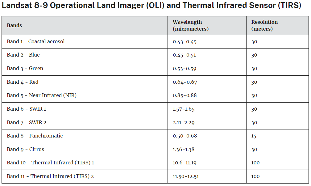
Figure 13.1. Landsat 8/9 band designations. Source: USGS https://www.usgs.gov/faqs/what-are-band-designations-landsat-satellites
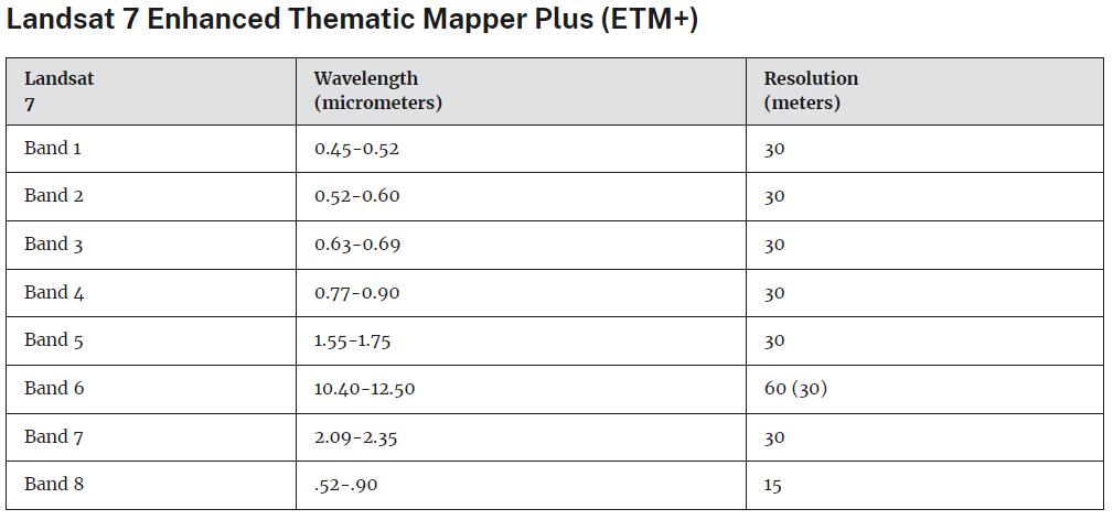
Figure 13.2. Landsat 7 band designations. Source: USGS. https://www.usgs.gov/faqs/what-are-band-designations-landsat-satellites
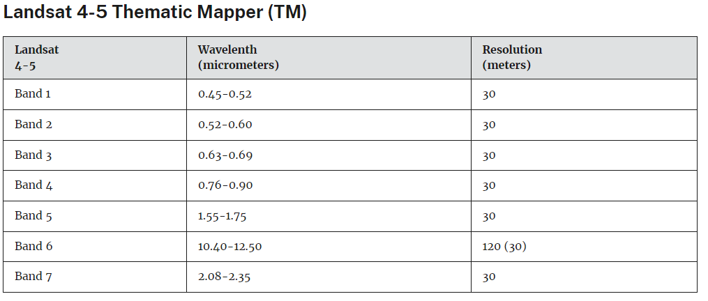
Figure 13.3. Landsat 4-5 band designations. Source: USGS. https://www.usgs.gov/faqs/what-are-band-designations-landsat-satellites
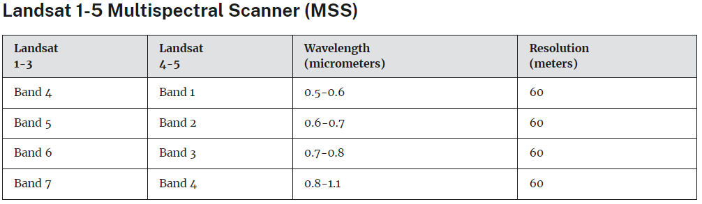
Figure 13.4. Landsat 1-5 band designations. Source: USGS. https://www.usgs.gov/faqs/what-are-band-designations-landsat-satellites
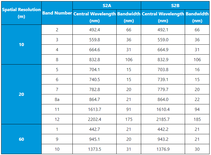
Figure 13.5. Sentinel spatial and spectral resolutions. Source: European Space Agency (ESA). https://sentinel.esa.int/web/sentinel/missions/sentinel-2/instrument-payload/resolution-and-swath
Adding Landsat 9 TIF files to ArcGIS® Pro
When the Landsat folder was unzipped, there were eleven individual TIF files, each associated with a separate band (Figure 13.6).
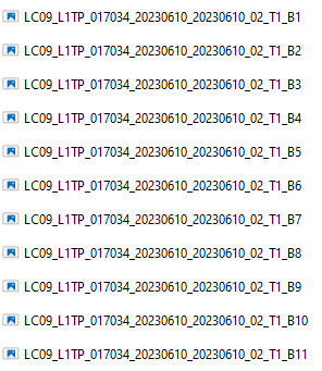
Figure 13.6. Each TIF file is associated with a separate band
Open ArcGIS® Pro and create a Map project. Name the project and navigate to your preferred folder on the computer to save it.
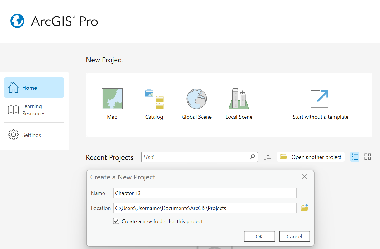
Figure 13.7. Opening a new project
Select the Map tab on the ribbon, and click the Add Data button in the Layer group.
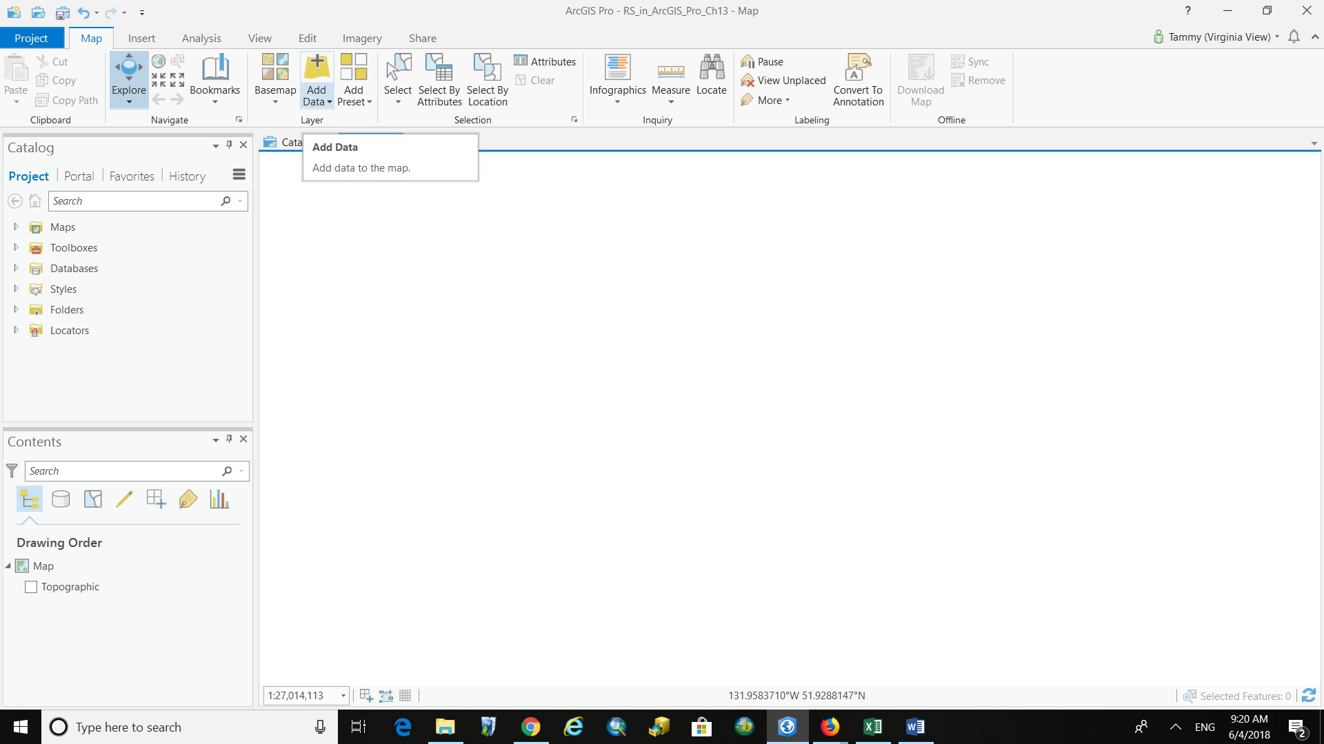
Figure 13.8. Adding data
Navigate to the folder where the unzipped Landsat TIF Files are located. Select the eleven TIF files named B1 through B11 and then OK to add them to the map project (Figure 13.9).
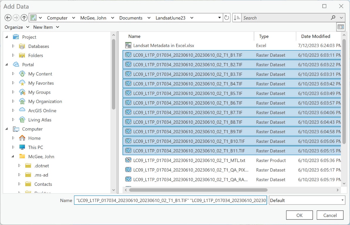
Figure 13.9. Adding the eleven TIF files
Calculate statistics for the image if prompted. Be patient while the files are added:
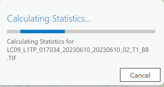
Figure 13.10. Calculating statistics
The images will appear in the ArcGIS® Pro map display and in the Contents pane (Figure 13.11).
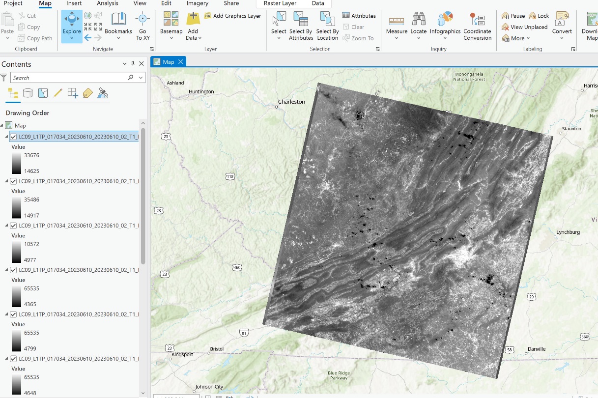
Figure 13.11. Landsat 9 images displayed in the map display
The eleven bands associated with the scene are listed in the Contents pane, stacked on top of one another.
Displaying Landsat Imagery in ArcGIS Pro
It is difficult to see all the TIF Files in Contents because the symbology is expanded for each image. Scroll down (red box in Figure 13.12) to view the additional images’ names and symbology.
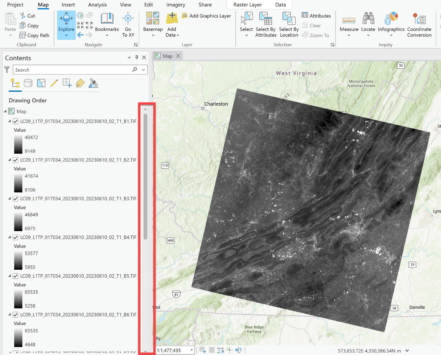
Figure 13.12. Using the scroll bar in Contents to access all images
The bands must be displayed numerically in Contents with band 1 on top, then band 2, band 3, and so on, as shown in Figure 13.12. If they are not displayed in that order, click and drag the images to rearrange them in numerical order.
Notice the name of each band in Contents is its Landsat Product Identifier, and the band number appears at the end of the name. The top layer is the one that is drawn last in the map display window and is therefore displayed on top of the others in the Map window (Figure 13.13).
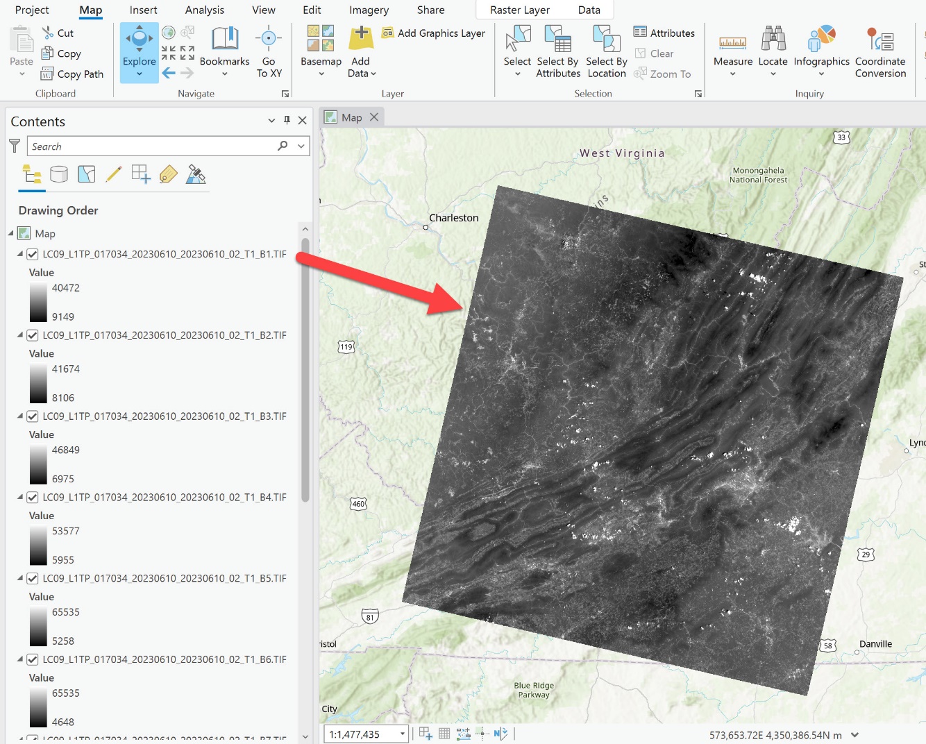
Figure 13.13. The top layer is contents is drawn last in the map display
As with vector layers and other raster layers, each band can be toggled off and on. It is possible to view bands displayed below other bands by unchecking those above the one of interest in the Contents pane. In Figure 13.14, we see band 3 in the map window because bands 1 and 2 are turned off (unchecked).
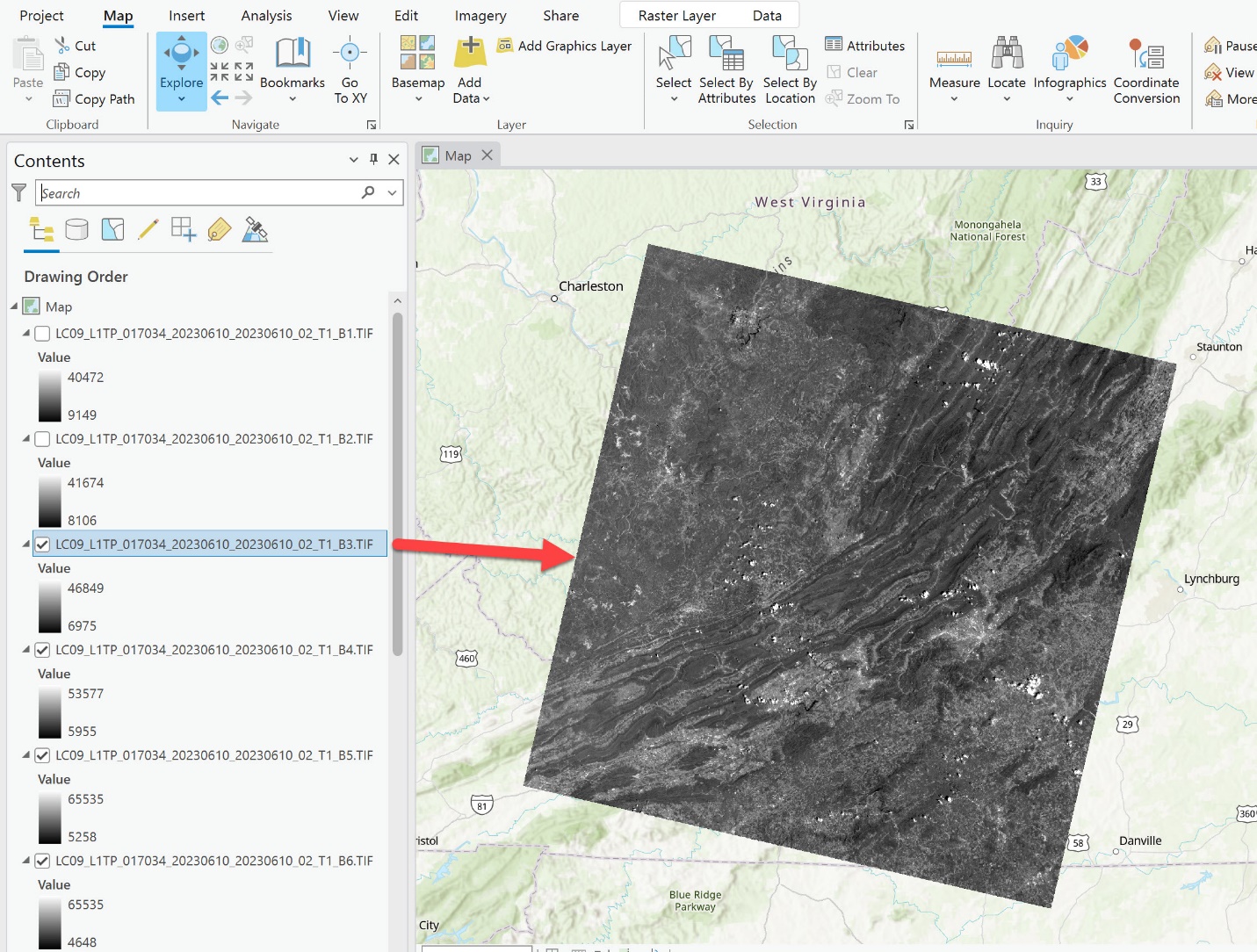
Figure 13.14. Turning off raster layers.
In Contents, to see all the layers listed without the need to scroll, collapse the symbology by clicking on the triangle icon to the left of the layer name.
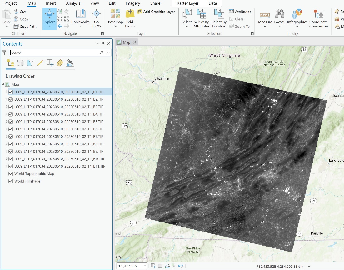
Figure 13.15. Collapsing symbology in Contents
Notice that each band is displayed in grayscale symbology. The digital number (DN) next to the grayscale reveals the range of brightness values within each band. In Figure 13.16, the brightness values for band 3 range from 6975 to 46849.
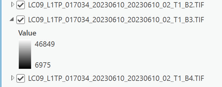
Figure 13.16. Brightness values of a raster image in Contents
Landsat 9 scenes are recorded in 16 bits, so each band ranges from 0 to 65,535 brightness values. (216 = 65,536 unique values, including 0). Brightness values refer to the reflectivity of the specific feature; the higher the number, the more reflective. (For more information – see Introduction to Remote Sensing by Campbell, Wynne, and Thomas, 2023.)
To view each band, uncheck the band layers starting with Band 1 and going down to Band 11. The topmost checked band is displayed in the map window. Each band appears slightly different in the map display because each contains data from a different region of the electromagnetic spectrum, and each band serves a different purpose.
Using Transparency and Swipe
We have all our layers turned on in Figure 13.15. Previously we turned the top layers off to see the next layer, but we can also leave two layers turned on and “see” beneath the top layer using a different technique. Turn off all layers except Bands 4 and 5. Be sure to have the image for Band 4 selected in the Contents pane and click on the Raster Layer tab that has appeared on the ribbon (Figure 13.17).
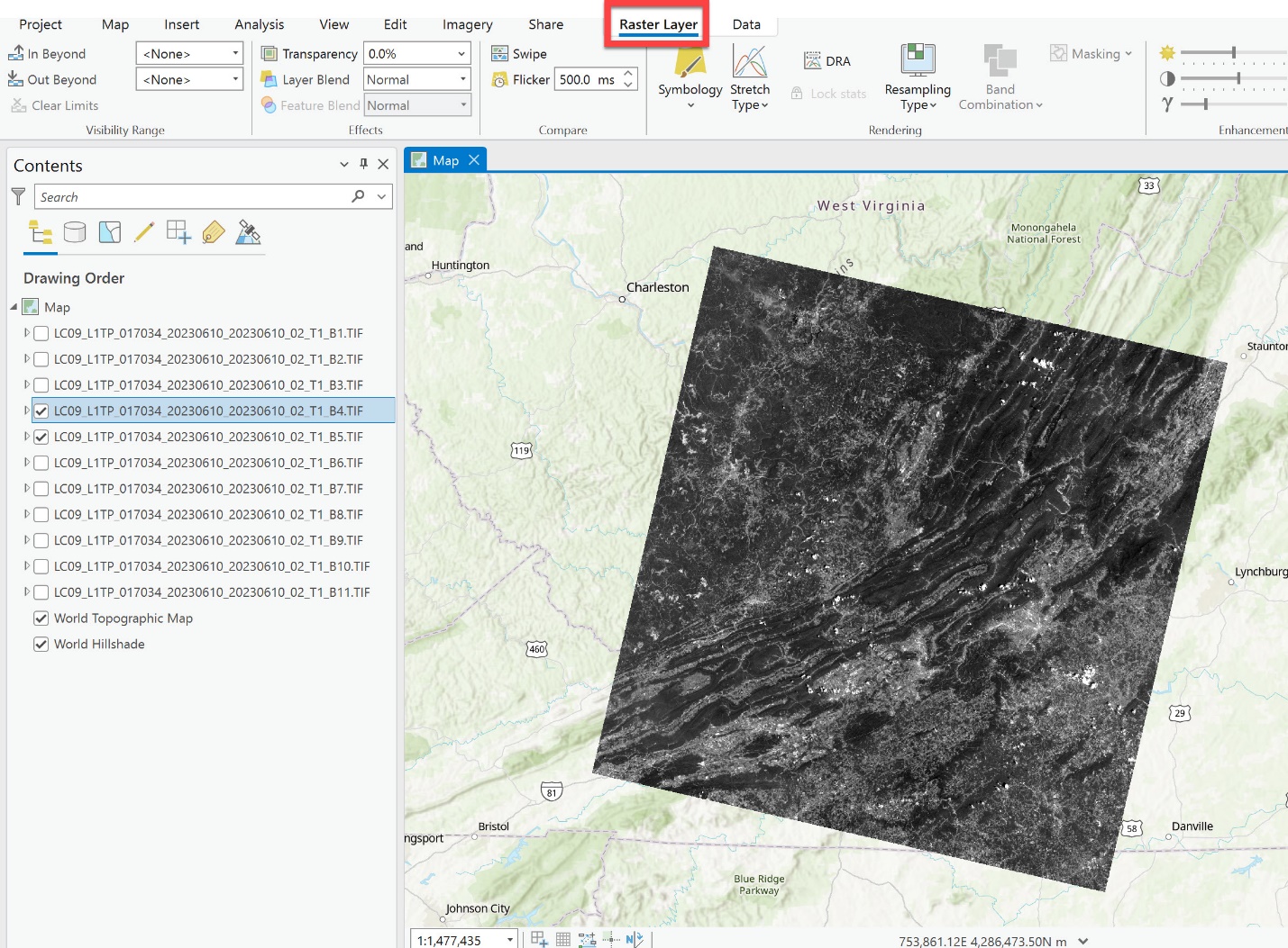
Figure 13.17. The Raster Layer tab
Two useful tools are on this tab: Transparency and Swipe (Figure 13.18).
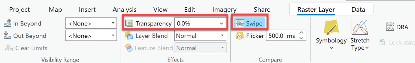
Figure 13.18. The Swipe tool
To change the Transparency of the topmost image, enter a value in the percentage box or click the drop-down and drag the slider to the desired percentage transparency. In grayscale, it is difficult to see any difference using transparency (Figure 13.19).
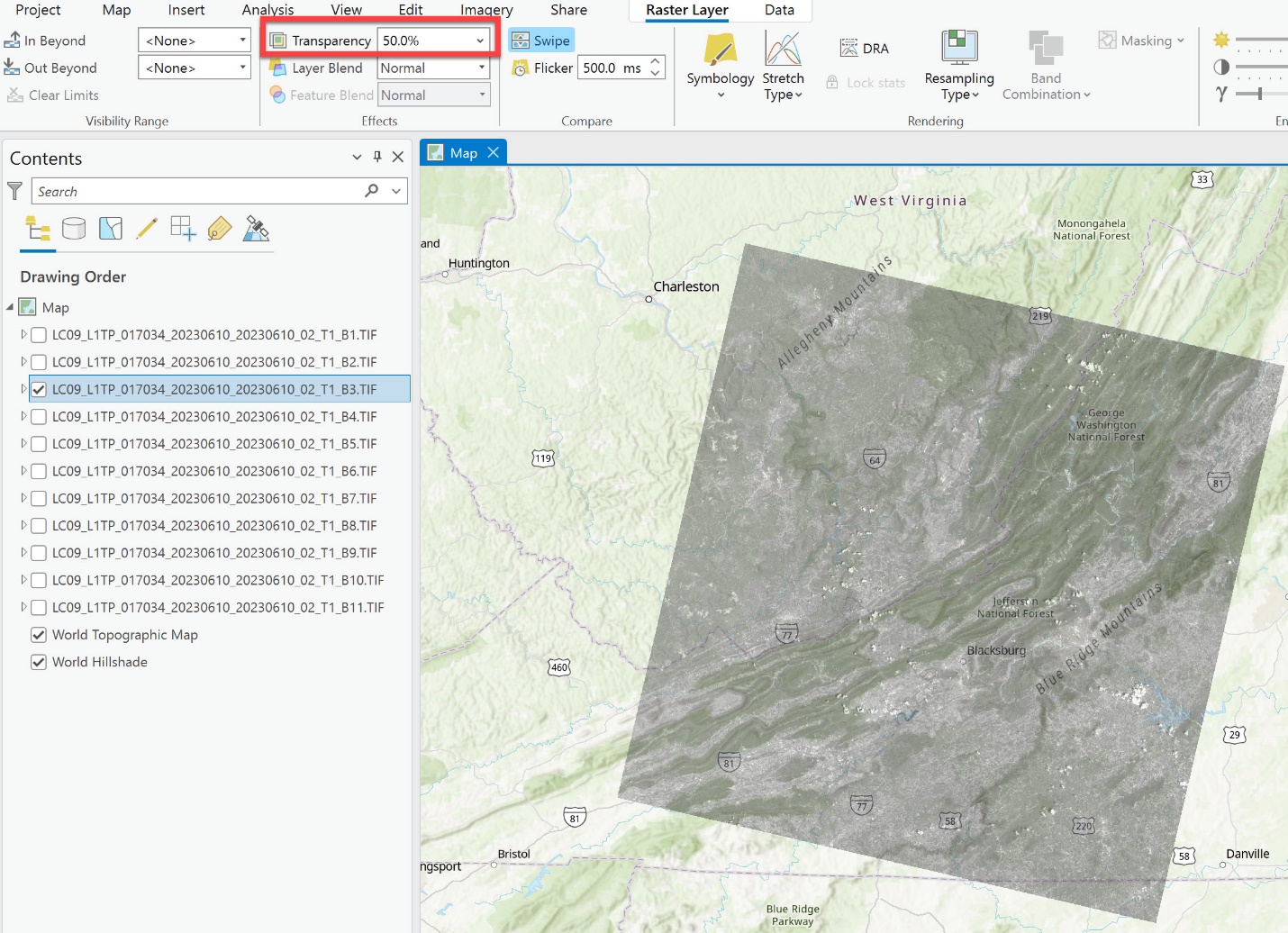
Figure 13.19. Setting transparency
However, even after changing the grayscale to another colored scheme1, it is still difficult to distinguish differences with transparency (Figure 13.20).
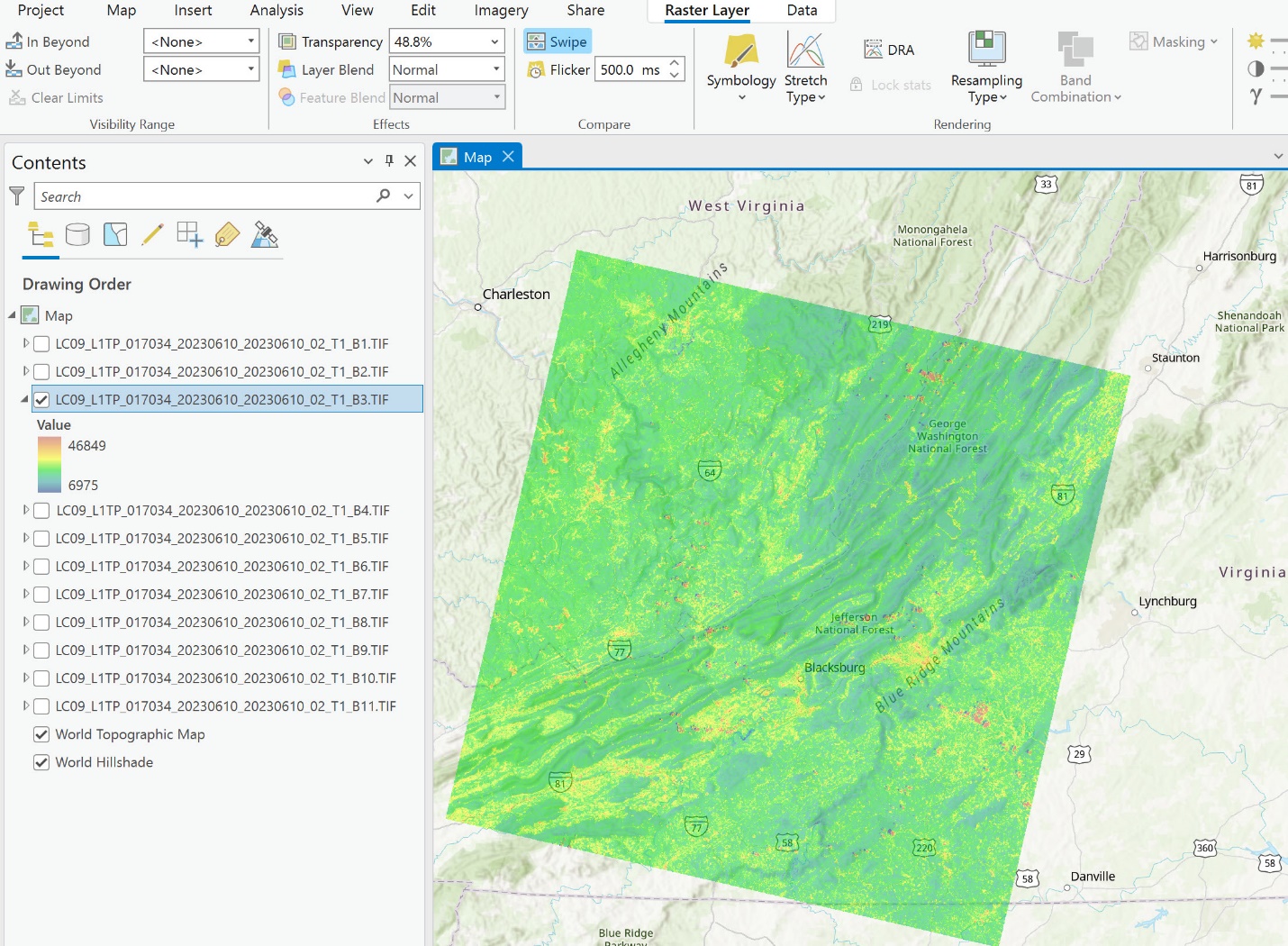
Figure 13.20. Changing grayscale to a different color scheme
The Swipe tool allows simultaneously viewing parts of two different images or layers. This tool works much better with images that share pixel boundaries. Select the top layer in the Contents pane and click the Swipe button. Place the cursor on the image and drag to reveal the corresponding image below the top one. (Figure 13.21).
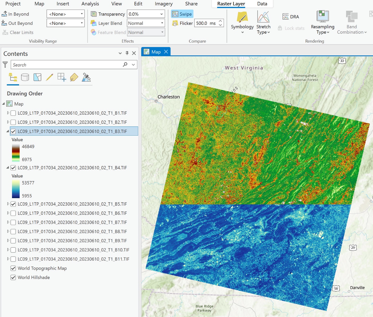
Figure 13.21. The Swipe tool
Swipe is an important tool that we will use in the last chapter, Chapter 23: Accuracy Assessment.
Metadata
We have introduced some readily available metadata and important tools for displaying the imagery. Now that the images are displayed, additional metadata is available.
Right-click on any layer name, select Properties, then Source in the left pane of the Layer Properties dialog box (Figure 13.22). Expand Raster Information to view the number of columns and rows for the image, that the image is one band, and the Cell Size X and Cell Size Y are 30. In Chapter 8: Metadata, we demonstrated how to find and interpret basic metadata elements. This is another way to view basic metadata for your image.
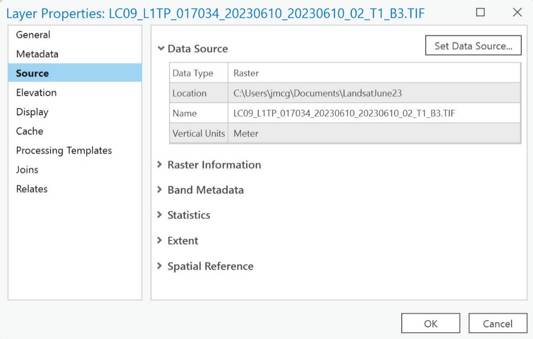
Figure 13.22. Accessing metadata
Expand Spatial Reference to view more detail such as the scene’s Projection, unit of measurement (Meters), and other details (Figure 13.23).
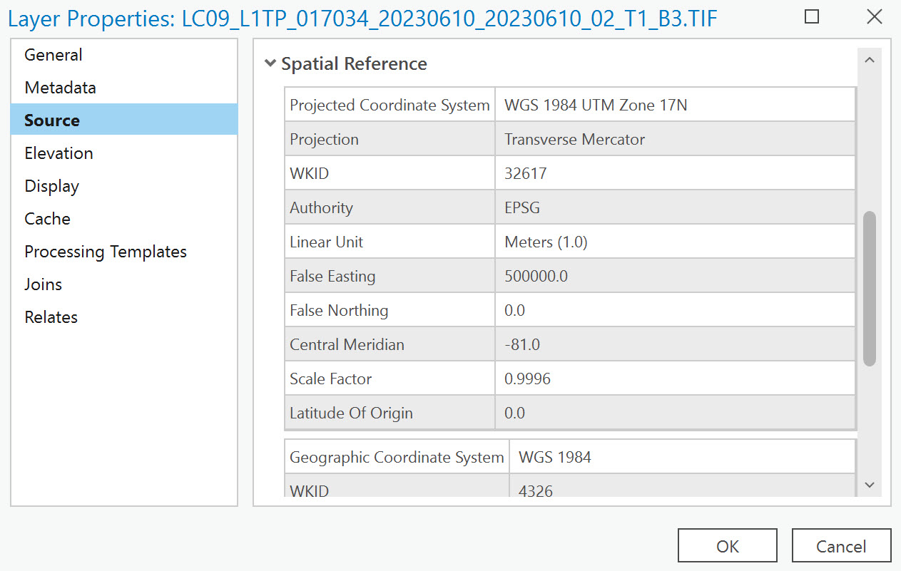
Figure 13.23. Metadata: Spatial Reference
Exploring Symbology
We already changed the symbology, but there is additional information about this image under symbology. Right-click on the same layer’s name and select Symbology.
The range of brightness values is shown to the right of Value (Figure 13.24). The Stretch type is Percent Clip, and the percentages used to calculate the stretch are in the Min and Max boxes.
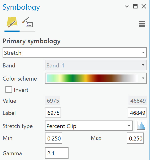
Figure 13.24. Setting the symbology stretch type
Stretch is the default Primary symbology for raster imagery. Other Primary Symbology types are Discrete, Classify, Unique Values, Vector Field (Figure 13.25). These are beyond the scope of this text, and we recommend that academic literature be consulted before using any of them for satellite imagery symbology.
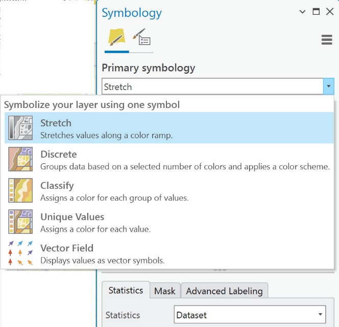
Figure 13.25. Primary symbology types
Drop down the options menu associated with Stretch type to view other selections (Figure 13.26).
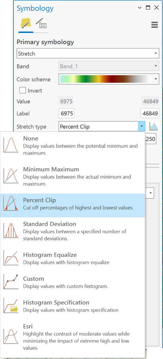
Figure 13.26. Symbology stretch type options
We will review some of these when we analyze imagery in subsequent chapters. But, if you are interested now, see ArcGIS® Pro help at http://pro.arcgis.com/en/pro-app/help/data/imagery/raster-display-ribbon.htm.
Summary
In this chapter, we demonstrated how to add the downloaded Landsat bands into ArcGIS® Pro, display them, change their order in the Contents pane, and identify areas of metadata. In the next chapter, Chapter 14: Creating a Composite Image for Landsat 9 Imagery, we will demonstrate combining multiple individual bands into a single composite image.