15 Chapter 15: Subsetting a Landsat 9 Composite Image
Introduction
Instead of an entire Landsat scene, the area of interest may be only one specific region within that scene or only particular bands. The previous chapter provided instructions on generating a single composite image of all eleven Landsat 9 bands. As previously discussed, a composite image can include three bands, four bands, or all eleven bands. This chapter provides instructions on how to limit the areal extent of the scene to a specific region (known as subsetting an image, or in GIS terms, clipping).
Getting Started
Create a new map project in ArcGIS® Pro and add bands 2 through 7 for the Roanoke, Virginia Landsat 9 image. Create a composite image for these bands using the geoprocessing tool introduced in Chapter 14: Creating Composite Imagery from Landsat 9 Imagery (Figure 15.1).
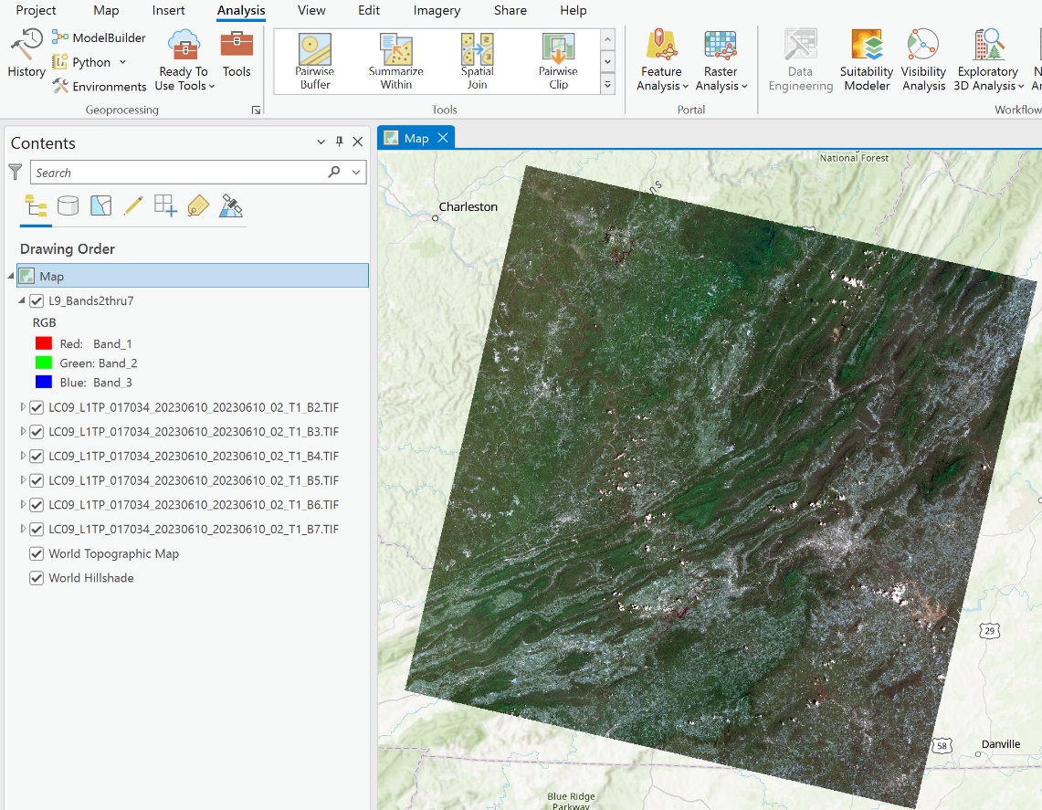
Figure 15.1. A composite Landsat 9 image in the map display
Why only these bands? From Chapter 14, Figure 14.1, these are the three visible (Blue, Green, Red), near-infrared (NIR), and short-wave infrared (SWIR) bands for Landsat 9 and are the only ones needed for our project. Why did we use the specific naming system for the new composite image? The name tells us that the bands included are 2, 3, 4, 5, 6, and 7, from Landsat 9 and the Roanoke area. So, when reviewing the band list in ArcGIS® Pro symbology for the composite image, we know the spectral band numbering sequence related to the renumbering done by the software (Figure 15.2).
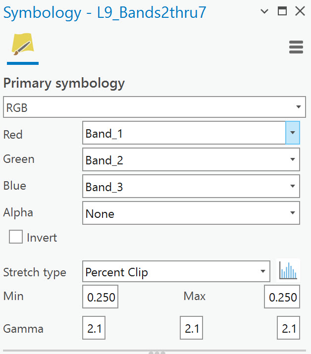
Figure 15.2. Assigning symbology to individual bands
We will use this new image for the subsetting exercise in this chapter.
Subsetting (clipping) by Spatial Extent
Limiting the spatial extent of this image can be accomplished in multiple ways. First, we will demonstrate the Export Raster tool. Select the composite image in Contents, then click the Data tab on the ribbon (Figure 15.3).
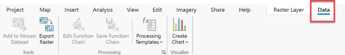
Figure 15.3. Data tab on the ribbon
Select Export Raster to open the tool.
Note that this tool is used for many purposes beyond subsetting. We will not review these other uses.
The composite image name automatically populates in the Output Raster Dataset box.
Expand Spatial Reference System and Clipping Options. Here is the Coordinate System where the projection can be changed if needed, but this option is beyond the scope of this book, so refer to the appropriate literature (Figure 15.4).
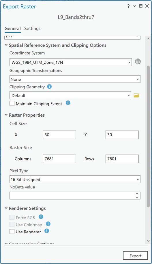
Figure 15.4. Exporting a raster
Click the down arrow for Clipping Geometry (used to subset an image). Several options are presented (Figure 15.5).
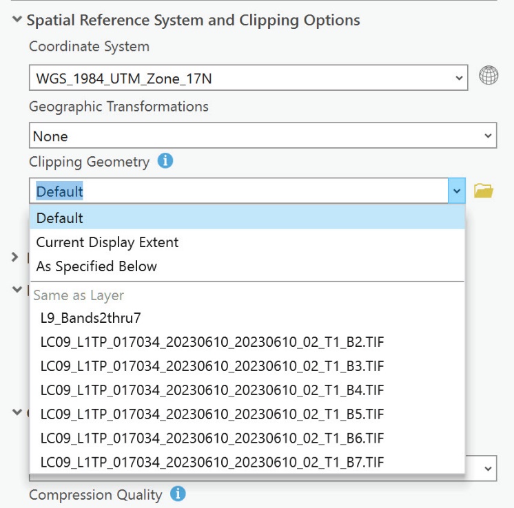
Figure 15.5. Clipping options
Default is used when making other changes, such as changing the coordinate system. That option will not be used in this chapter.
Current Display Extent—use this setting if the image in the map window is zoomed in to a specific region. This is the option that will be used in the example below.
As Specific Below—use this setting if the specific coordinates for each corner of the desired region are known. We will also demonstrate this.
The next item is Same as Layer, listing the name of our composite image and the individual bands used in the compositing. These are the names of the layers that are present in the project. You can add a layer, such as a vector feature class or shapefile, with the boundaries of your study area and choose that file as the option for Subsetting. We will also demonstrate this option below.
The Export Raster tool is used to change any raster’s parameters and export it to a new dataset. We are only subsetting to an areal extent (clipping the image) for our purposes.
To examine a few other parameters that populated when the tool opened. Under Raster Properties, Raster Size is the number of pixels in Columns and Rows present in the image. The values in these boxes represent the entire scene.
Under the Renderer and Compression Settings are additional options. We will leave these as default—many of these are used for other types of processing.
Note: Our purpose here is not to evaluate the results from each type of setting but to provide the basics for accomplishing the subsetting task. Refer to ArcGIS® Pro Help and current literature to determine if your project requires other settings.
Clipping to the Extent of the Current Display
Now that we have reviewed the tool let’s set some parameters. First, we are going to clip to the extent that is displayed in the map viewer. Zoom in on the area of the image that includes the city of Roanoke (white circle), the Christiansburg/Blacksburg area (red circle), and Smith Mountain Lake (blue circle) (Figure 15.6).
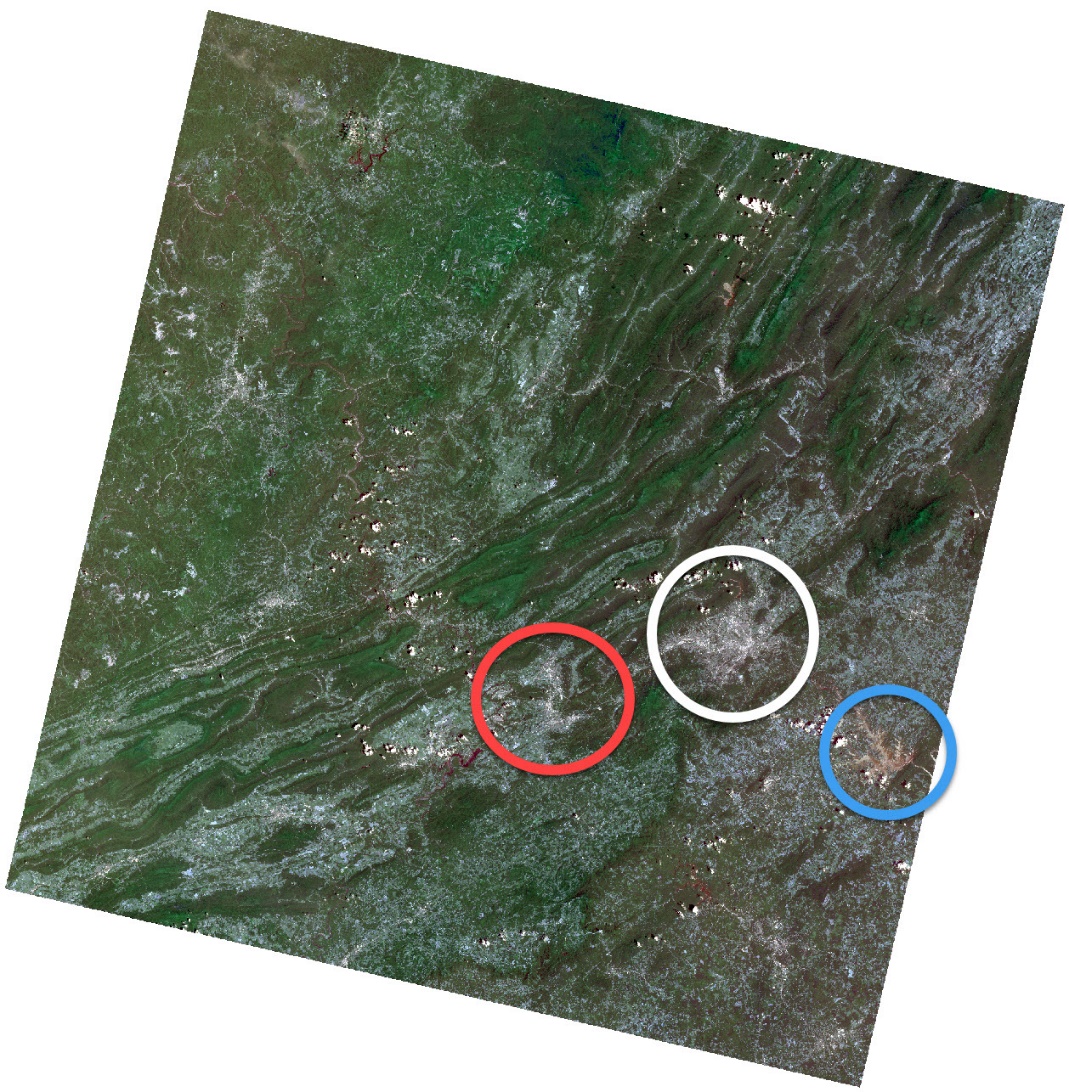
Figure 15.6. Areas of interest
When zoomed in, it should look like Figure 15.7.
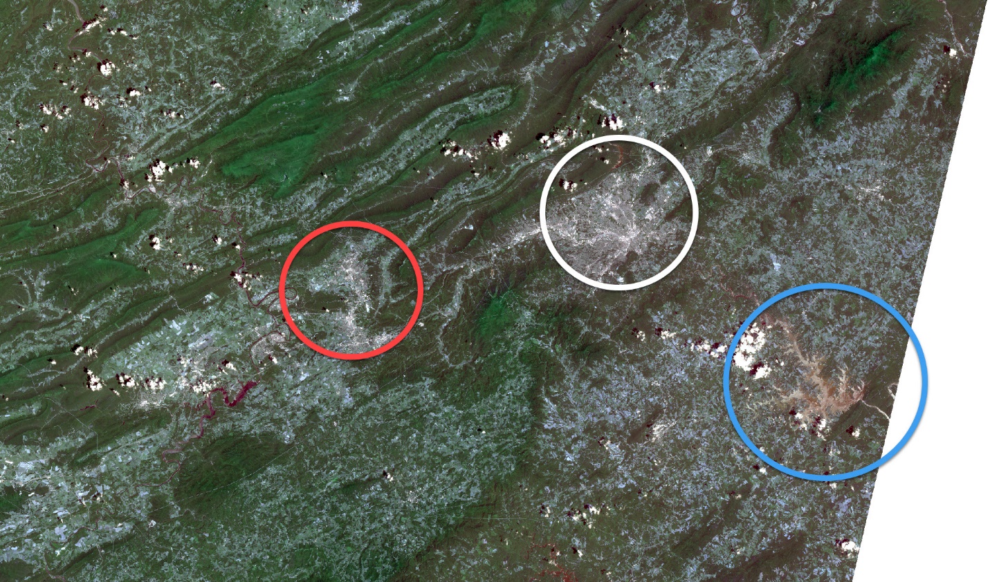 Figure 15.7. Zooming in to the areas of interest
Then, within the Export Raster tool, under Spatial Reference System and Clipping Option, choose Current Display Extent from Clipping Geometry. ArcGIS® Pro automatically changes it to As Specified Below and adds the coordinates to limit the extent (Figure 15.8).
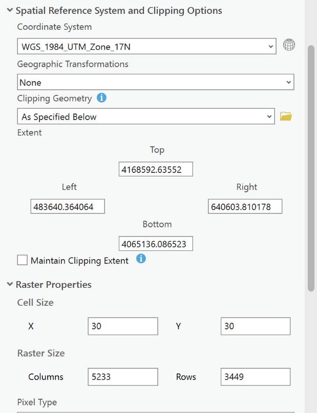
Figure 15.8. Clipping geometry
Compare the number of Columns and Rows in Figure 15.4 (7681 and 7801) to Figure 15.8 (5233 and 3449). We are clipping the scene to a smaller areal extent. Leave all other parameters as Default and click Export. The processing progress bar is indicated at the bottom of the tool.
When finished, a new layer with the same name as the composite but with a .tif extension will be at the top of Contents, and a new image will be displayed in the map window (Figure 15.9).
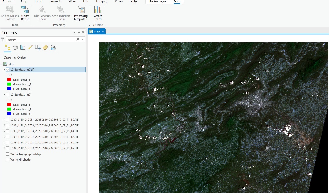
Figure 15.9. A new image is displayed in the map window
Close the Export Raster pane and turn off the original composite image. Right-click on any of the individual Landsat band images and choose Zoom to Layer to confirm that the image is a subset of the original extent (Figure 15.10).
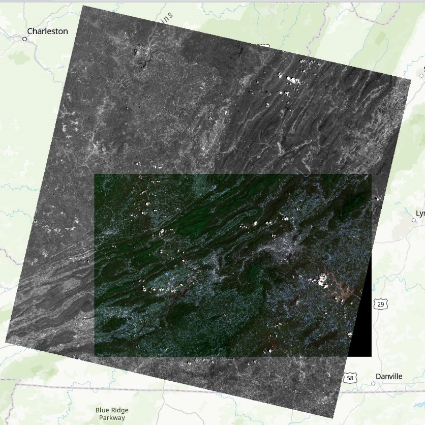
Figure 15.10. Comparing the clipped image with the original image
Do this process again (use the original composite) but limit the extent to that for just Roanoke, Virginia.
The results should be similar to Figure 15.11.
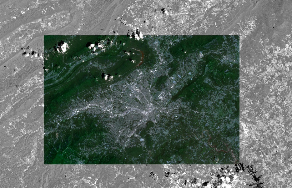
Figure 15.11. The subsetted image.
We will show two additional methods of clipping.
Clipping Using a Polygon
Another clipping option is to clip to an existing polygon.
To do this, we will add a polygon vector shapefile that represents the spatial extent of the area desired. In this example, we have added two polygon shapefiles to demonstrate the process— Montgomery County, Virginia, and a square around Roanoke, Virginia (Figure 15.14).1
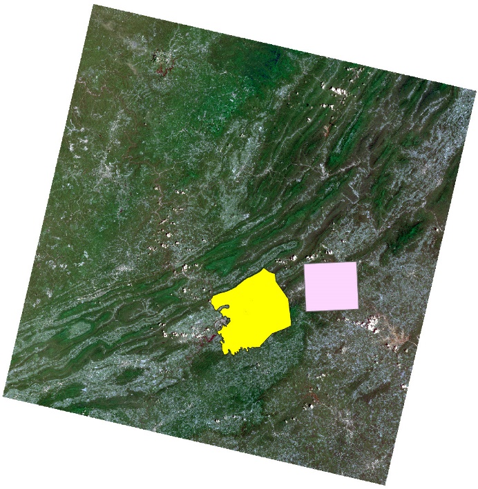
Figure 15.12. Clipping using a polygon
Again, select the original composite image in Contents. Open the Export Raster tool from the Data tab on the ribbon. As shown in Figure 15.13, change the name of the output raster to reflect Montgomery County and choose the MontgomeryCoVa file for Clipping Geometry. Make sure that the box is checked next to Use input features for clipping geometry.
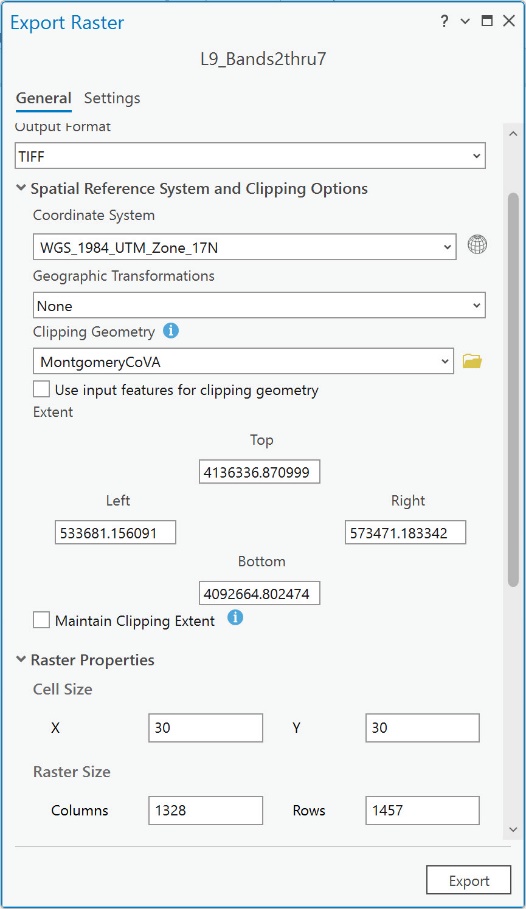
Figure 15.13. Clipping using a polygon
Leave all other settings as default and click on Export. Once the tool runs, you again see a new file in Contents and have a new image in the Map viewer (Figure 15.14).
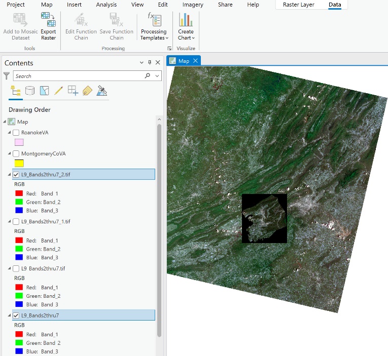
Figure 15.14. A clipped image
Notice, however, it is more than the county outline. The dark pixels surrounding the Landsat scene are not brightness values. This is the GIS’s attempt to make the image have the same areal extent at its corners. These outer border areas are black because the cells have “no data” associated with them. These black borders can be hidden, but you must change the settings before subsetting the image.
Click on Project, Options, Raster and Imagery and expand Appearance. Check the box before Display Background Value and set it for No color and the same No color for NoData (Figure 15.15). Click OK. Click on the back arrow in the upper left to return to your project2.
Figure 15.15. Settings for NoData
Now let’s do the subset one more time for MontgomeryCoVA. The NoData pixels are not displayed (Figure 15.16).
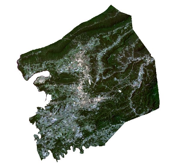
Figure 15.16. NoData pixels are not displayed
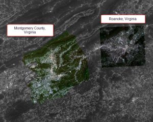
Now do the process again using the shapefile for Roanoke, Virginia, ensuring the original composite image is selected before setting the Clipping Geometry and running the tool. Figure 15.19 shows the subsetted images from Montgomery County and Roanoke, Virginia.
Figure 15.17. Map display showing subsetted images
We used the same composite image for subsetting both areas. Why do the images look different in color? When subsetting, we may reduce the variation in brightness values so the ranges across which the values are displayed in the two images differ (Figures 15.18 and 15.19).
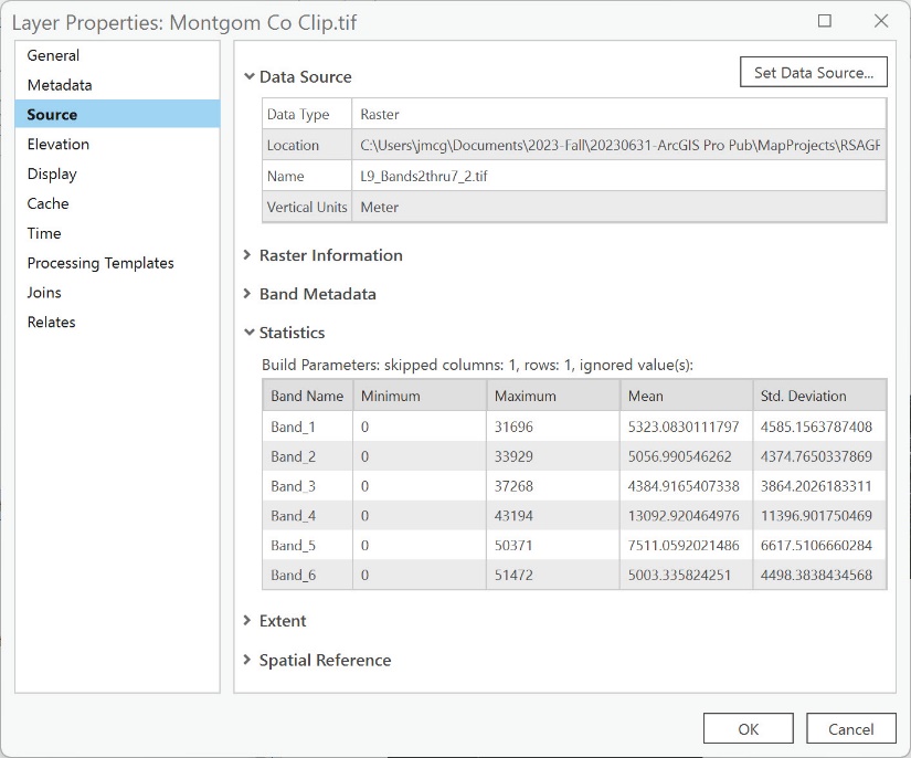
Figure 15.18 Statistics for Montgomery County Subset
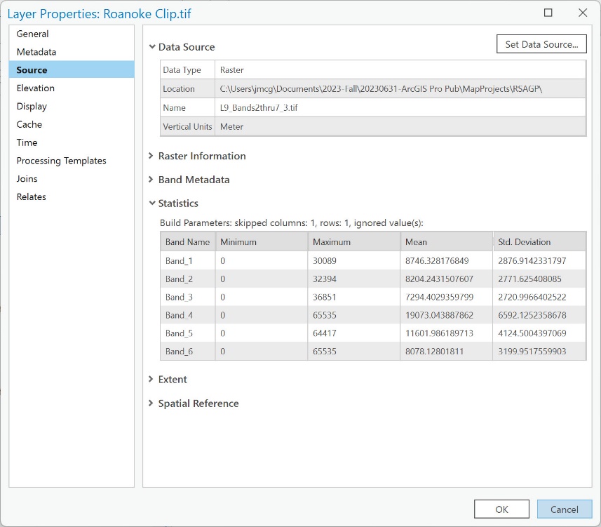
Figure 15.19 Statistics for Roanoke Subset
Creating a Composite Image and Clipping in One Step
We are going to demonstrate one more process. Creating a composite image and clipping can be done at the same time. However, the results are different, as we will show. In this method, we will use the Processing Extent.
Go to the Analysis tab, and choose Environments from the Geoprocessing group. Choose the file with the desired extent (the area of interest) from the Extent drop-down under the Processing Extent category. (Figure 15.20). We will select Montgomery County, Virginia.

Figure 15.20. Creating a composited subsetted image in one step
Once we choose Montgomery County, Virginia, ArcGIS® Pro populates the coordinates for that extent (Figure 15.21). Click OK.
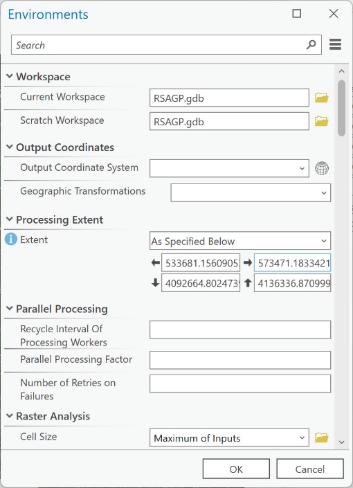
Figure 15.21. Creating a composited subsetted image in one step.
Now, open the Composite Bands geoprocessing tool, and redo the composite (if you forgot how to accomplish this, return to the prior chapter). For this example, we use Bands 2-5 (Figure 15.22). Once populated with the bands and the output raster has a name, click Run.
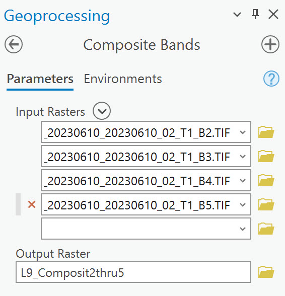
Figure 15.22. Creating a composited subsetted image in one step.
The new clipped image is a rectangle, not the shape of the county outline, as it was in the previous clipping method (Figure 15.23). In Environments, when we chose the Montgomery County shapefile as the input, it clipped using the upper left corner coordinate, upper right corner coordinate, lower left coordinate, and lower right corner coordinate, which resulted in a rectangle.
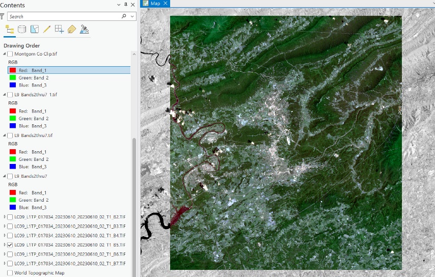
Figure 15.23. Results in the map display.
Of the methods we demonstrated, which approach is better? There is no right or wrong answer, as this is contingent on the project’s parameters. One approach provides a subset of a general region. The other approach offers a subset of a more specific user-defined extent, which could include irregular boundaries such as a watershed or political boundary.
Please note this caution. When we demonstrated these processes for subsetting an image, in most cases, we left it up to ArcGIS® Pro to provide a name for each new raster. This might be confusing as the layers pile up in contents, especially determining which layer statistics to review when discussing Figures 15.20 and 15.21. We were manually documenting as we did each process. It is better to choose specific names to help distinguish between the different images or go to their metadata and manually enter the information.
Please proceed to the next chapter, Chapter 16: Band Combinations Using Landsat 9 Imagery.