21 Chapter 21: Unsupervised Classification of a Landsat 9 Image

Introduction

Image classification is a process that sorts individual pixels based on their spectral values into informational classes or categories. A pixel is assigned to a class corresponding to a specific set of criteria. Two methods to classify individual pixels are:

• Unsupervised Classification (this chapter)
• Supervised Classification (Chapters 22 – 24)

With unsupervised classification, the pixels are clustered together based on spectral homogeneity and spectral distance. Spectral homogeneity is evaluated by the software program—in this book, ArcGIS^® Pro. Spectral distance is measured using various techniques chosen by the analyst. Unsupervised classification produces classes of homogeneous spectral identities that may not exactly correspond to informational classes. While spectral classes denote pixels grouped by uniform brightness values, informational classes refer to groups that convey useful information with designations such as land use, soil classes, or agricultural productivity. When using unsupervised classification, the informational class may contain a variety of spectral identities. Therefore, a spectral class identified by unsupervised classification seldom matches exactly to an informational class.

ArcGIS^® Pro accomplishes unsupervised classification using ISO Cluster. ISO is an algorithm in which a mean is derived from the spectral values for the input bands. Variance and co-variance are also calculated. The algorithm automatically recalculates the statistical values as pixels are added to each spectral class. 

Objectives for this Chapter

The objectives for this chapter include:

• Complete an unsupervised classification on a Landsat 9 image.
• Determine the land use/landcover category associated with each spectral class.
• Create color-coded informational classes according to the following scheme:

• Calculate the percentage of the total area for each informational class.

Conducting Unsupervised Classification

Please open a new project, name it, save it, and add the 6-band composite image created in Chapter 15—the image that was clipped to the extent of the display. Set your workspaces and eliminate background values. To help discern features, set it to a natural color band combination (Figure 21.1).

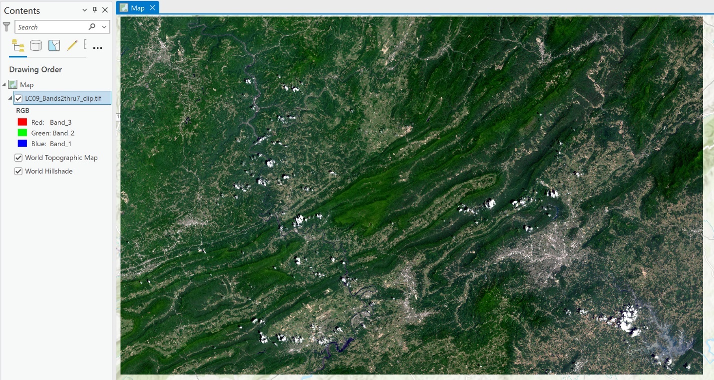
Figure 21.1. True color Landsat 9 image

As with all other processes, there are multiple ways to complete the unsupervised classifications. One method is to use the Classification Wizard from the Imagery tab on the ribbon (Figure 21.2). However, as with many other shortcut functions, this creates an image only usable in the current map document.

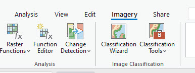
Figure 21.2. The classification wizard

The method demonstrated in this chapter will create a permanent image usable in other analyses, and we will use this image in the final chapter—Chapter 25: Accuracy Assessment. Go to the Analysis tab, Tools, and in the Geoprocessing pane, search for Classification (Figure 21.3).

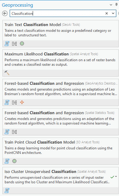
Figure 21.3 Classification options

We want ISO Cluster Unsupervised Classification (Figure 21.4).

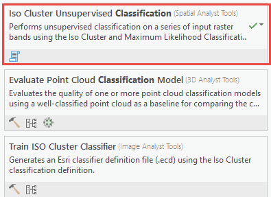
Figure 21.4 The ISO Cluster Unsupervised Classification Option

Figure 21.5 shows the tool and the inputs required. Before we proceed, we will discuss some of the inputs.

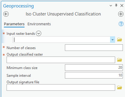
Figure 21.5. ISO Cluster Unsupervised Classification

Under Input raster bands, choose the 6-band subsetted composite image (Figure 21.6). This tool is set up so if you do not have a composited image and only individual bands, you can choose the bands you want to use in the classification process. Since you are following the procedures demonstrated in this book, you will use a multi-band image created in prior chapters.

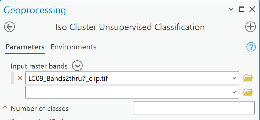
Figure 21.6. ISO Cluster Unsupervised Classification

Determining the Number of Classes

Remember from the first page of this chapter, for our final output, we want four different informational classes:

 

The number of classes in the ISO Cluster Unsupervised Classification dialog box refers to the number of spectral classes. Set this number to 25. Why? The image has over 65,000 different pixel values. Each category of features or informational classes—water, agriculture, urban, forest—may consist of a range of spectral values. Unsupervised classification generates groups of pixels that form homogenous spectral identities. The number of spectral classes used will depend on the number of informational classes, the complexity of the area of interest, employer or government requirements, and the goals of the analysis. Determining the appropriate number of spectral classes may require running the ISO Cluster Unsupervised Classification tool multiple times using different numbers of spectral classes. Other parameters may also be necessary, but let’s leave these parameters at their default settings for our demonstration.

As noted above, set the Number of classes to 25 and leave all other parameters as default (Figure 21.7). The Minimum class size refers to the smallest number of pixels the software should place in one spectral class. Name the Output classified raster something recognizable for the process and ensure it will be stored in the geodatabase for the project. Then Run the tool.

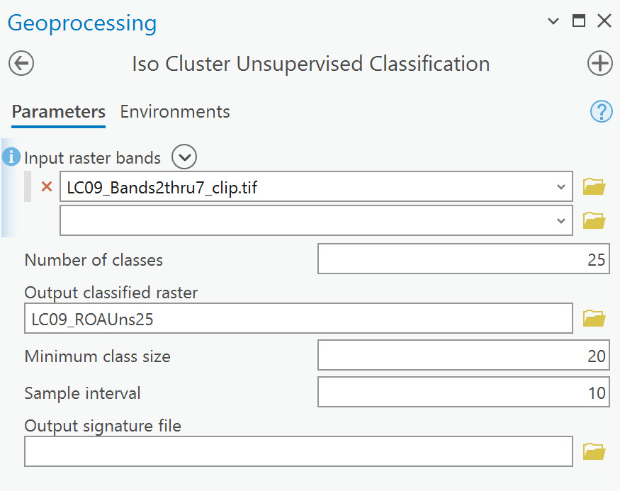
Figure 21.7. ISO Cluster Unsupervised Classification

The classification process takes a few minutes. But when it is complete, a green message appears at the bottom of the tool (Figure 21.8).

Figure 21.8. Classification complete

A new layer appears in Contents, with its image in the map viewer (Figure 21.9). Because the number of classes was set to 25 clusters of spectral values, there are 25 unique values in the symbology. Colors have been randomly assigned to the new image of homogenous spectral classes (not informational classes).

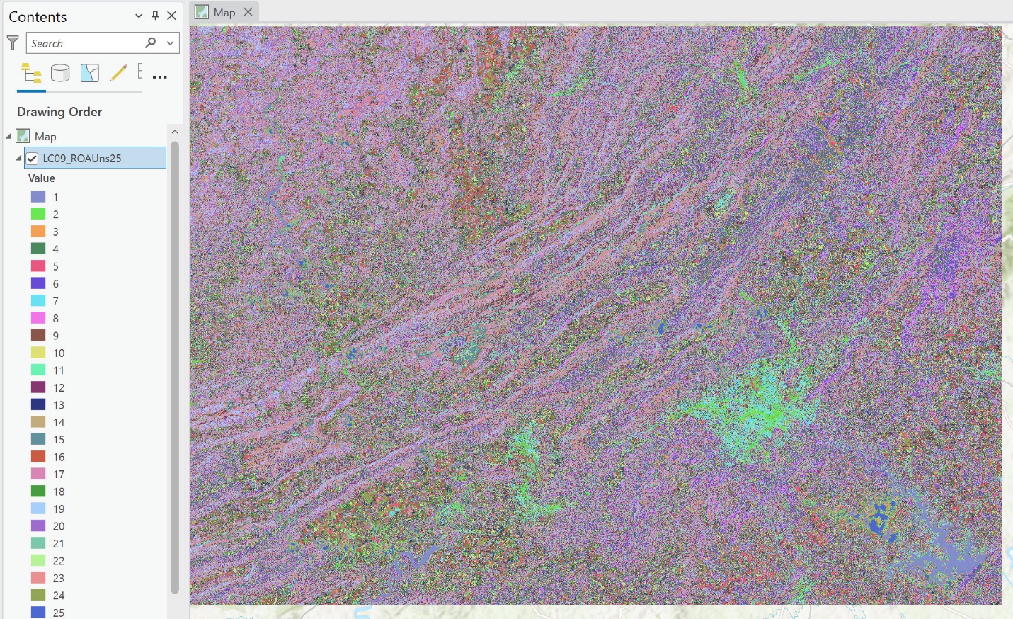
Figure 21.9. Classes with randomly assigned colors

We must determine which spectral class(es) should be assigned to each informational class. All 25 spectral classes will ultimately be assigned to one of our four designated informational classes. Don’t forget to save your project regularly!

But before we do this, let’s rerun the classification method to see what happens when the number of classes changes. Set the number of classes to 50, name the Output classified raster, and Run the tool (Figure 21.10).

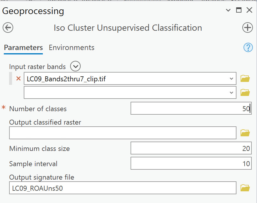
Figure 21.10. Unsupervised classification dialogue

As before, a new layer appears in Contents and a new image in the map viewer (Figure 21.11). This time, 50 unique values and colors are assigned to the new image of homogenous spectral classes (not informational classes). If your image is symbolized as shown in Figure 21.11, that is ArcGIS^® Pro using a stretch symbology for ease of display.

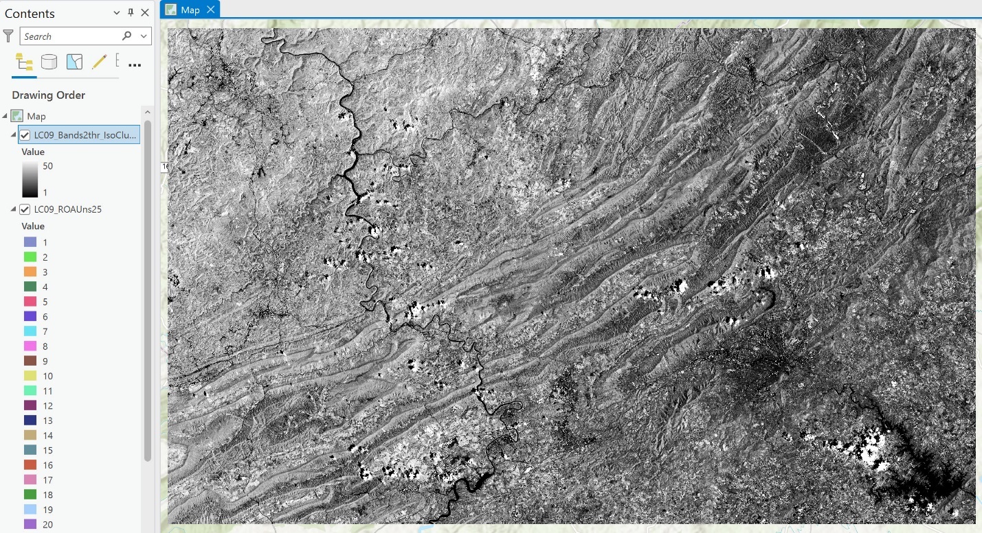
Figure 21.11. Greyscale stretched symbology

This is changed to Unique Values under Symbology (refer to Chapter 7 if you need a refresher). In Figure 21.12, we changed the symbology to Unique Values.

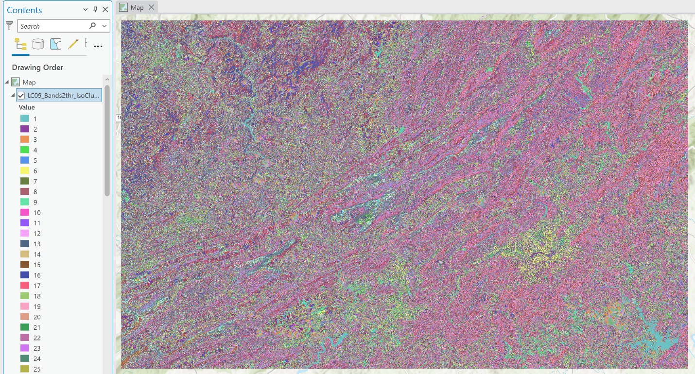
Figure 21.12. Classes assigned to unique values

As previously noted, the number of spectral classes chosen depends on many factors. For this image and its variation in land use, 50 classes are likely more appropriate than 25, but the number of classes is often contingent on the specific application.

Classifying the Unsupervised Clusters

Now we need to decide which informational class contains each spectral class. Which classified image will we use? From here on, we will use the image with 25 spectral classes strictly for simplicity and instruction. For real applications, 50 spectral classes should be used, if not more.

 

Add a new base map layer, Imagery, to help decide which spectral classes belong to a particular information class. (Figure 21.13)

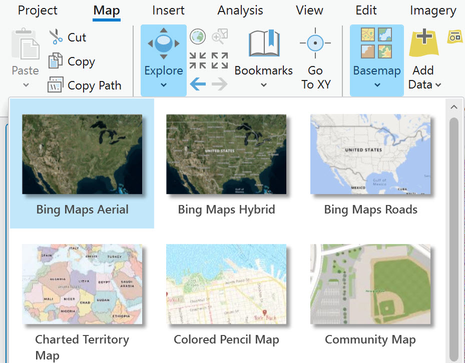
Figure 21.13. Base map options

This base map looks similar to our natural color composite. Drag the image with 25 spectral classes to the top of the Contents (we will call this image Unsupervised 25 from here forward) or turn off the image with 50 spectral classes. Also, turn off the original composite image(Figure 21.14). You can also use  the Swipe  tool to compare the classified image with the Imagery base map.

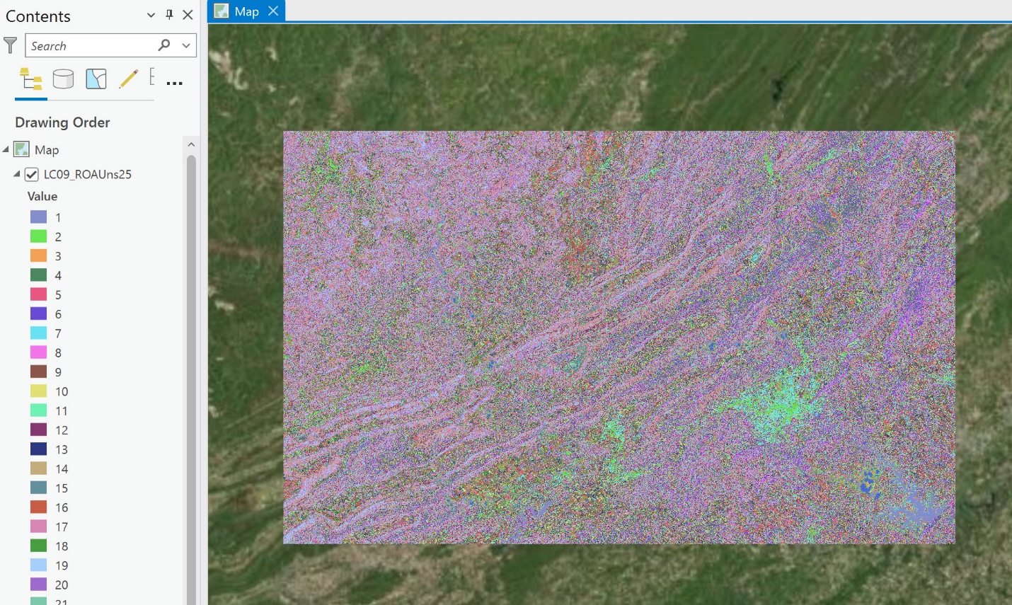
Figure 21.14. Classified image superimposed over the imagery base map

The base map image appears also to be a satellite image. As you zoom in, it changes to higher-resolution aerial imagery, which will be needed to help determine the specific informational class for each pixel in the image (Figure 21.15).

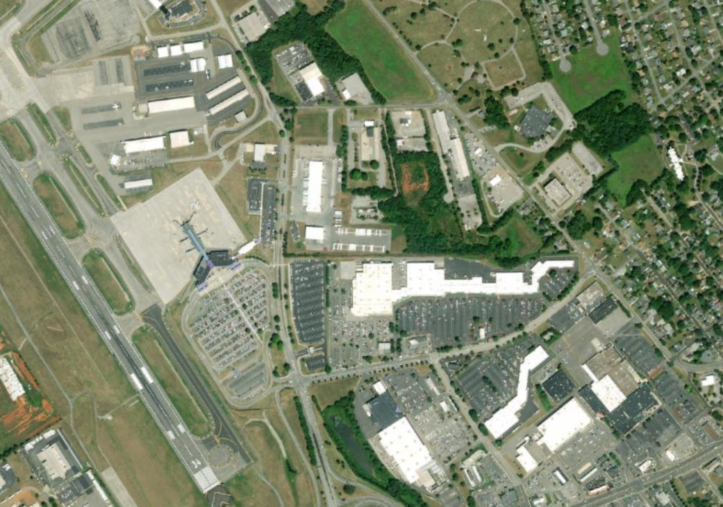
Figure 21.15 Basemap imagery zoomed into an area in Roanoke, Virginia

For your first step, please change the color for any spectral class that has any of our final informational color classes (red, yellow, green, blue) to any other color. This would eliminate confusion if any of the spectral classes were assigned by default (by ArcGIS® Pro) to a class color in our scheme. Alternatively, you could begin by setting them to all the same color and then proceed.

To change the spectral class color, start with water. Water is symbolized as blue, so zoom in to Smith Mountain Lake to determine the pixel value and color (again, ensure the blue you use is not a color showing as a symbol used in Contents). Click on a pixel to check the pixel value (Figure 21.16). As a reminder, since this is a classified image, pixel values are not associated with brightness values but have been assigned a classification value. The pixel value of your unsupervised classification (25 classes) will therefore range from 1 to 25. This shows its Pixel Value is 1.

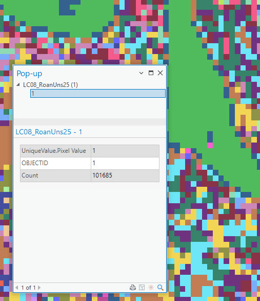
Figure 21.16. Exploring pixel values

In Contents, find that value under the layer name, right-click on the symbol, and change it to blue. In Figure 21.17, we chose Lapis Lazuli.

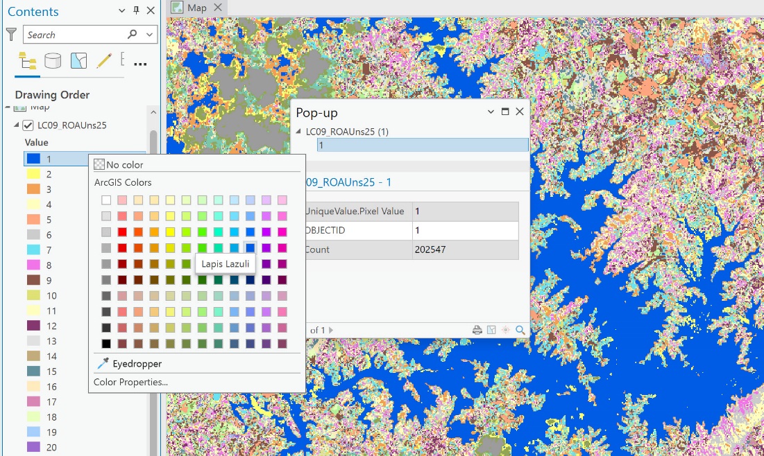
Figure 21.17. Assigning blue to water clusters

All water pixels’ spectral values will be assigned to blue. In this case, class one is associated with water, so we are changing all the pixels with a value of one to blue for the water information class. Once the color is chosen, it changes the color in the map viewer (Figure 21.18).

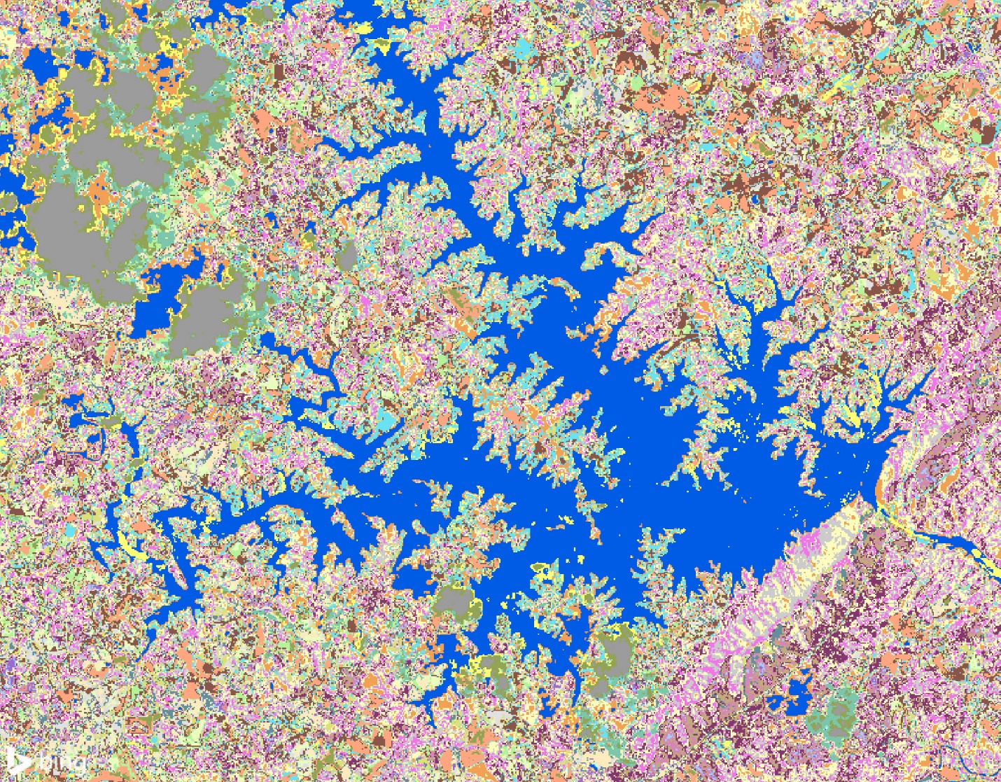
Figure 21.18. Assigning blue to water clusters

Notice in our image that some of Smith Mountain Lake is also other colors. Use the Swipe tool to verify that those colors are also water within the lake (Figure 21.19). If yes, then change that specific pixel value also to Lapis Lazuli.

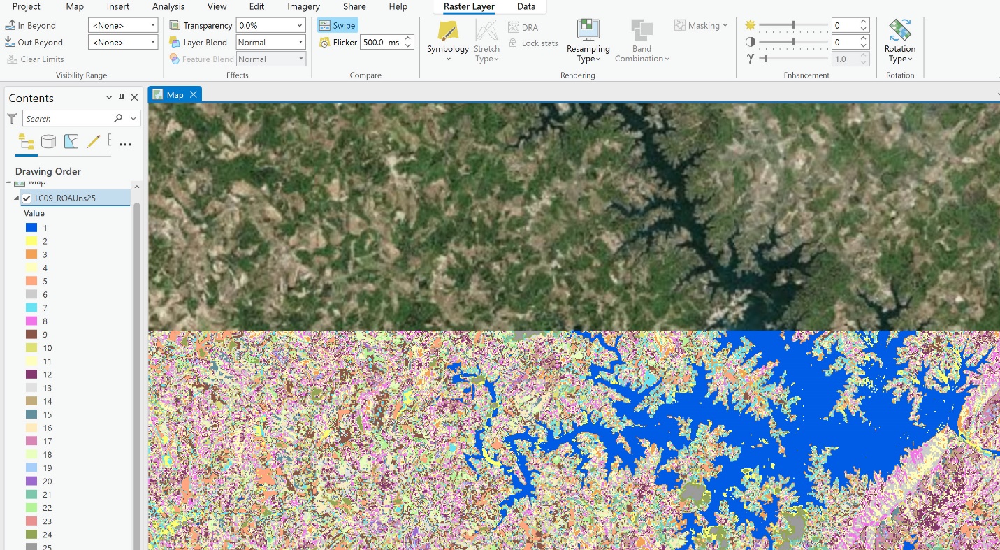
Figure 21.19. Using the swipe tool

Zoom to the rivers in the Roanoke and Radford areas and change their colors to the same blue if they still need to be changed. To find the river in Roanoke, follow the blue water northwest out of Smith Mountain Lake. But be careful since we only have 25 spectral classes—mountain shadows and cloud shadows can mimic water.

Continue with the other spectral classes – all 25 classes must be evaluated and assigned to the appropriate color class.

Associate agriculture fields with yellow (Figure 21.20).

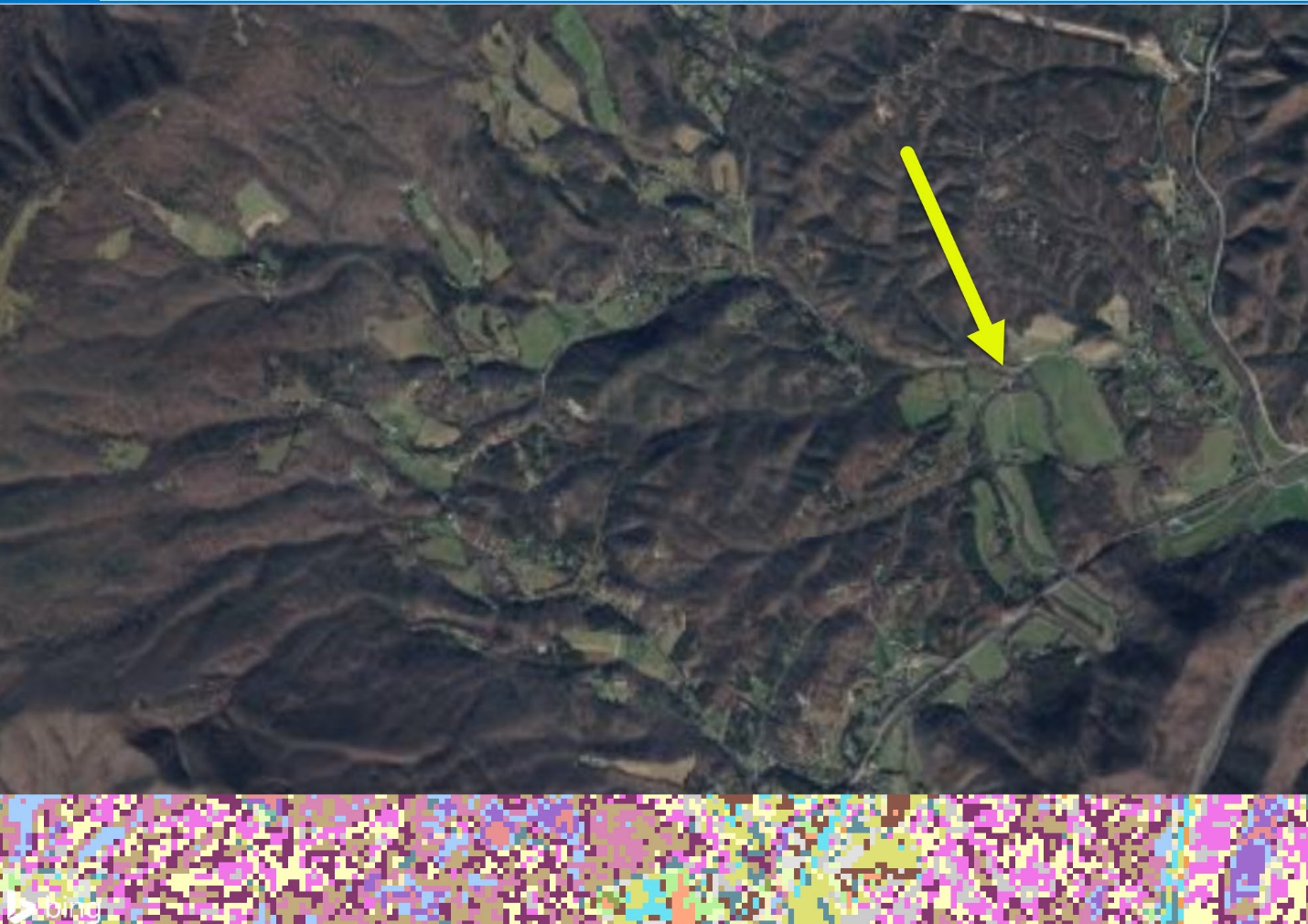
Figure 21.20. Associating agricultural fields with yellow

Associate forests with green (Figure 21.21).

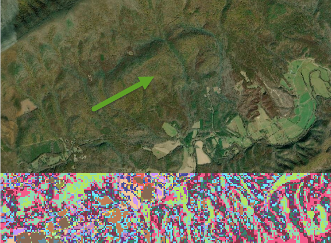
Figure 21.21. Associating forests with green

Urban areas should be red (Figure 21.22).

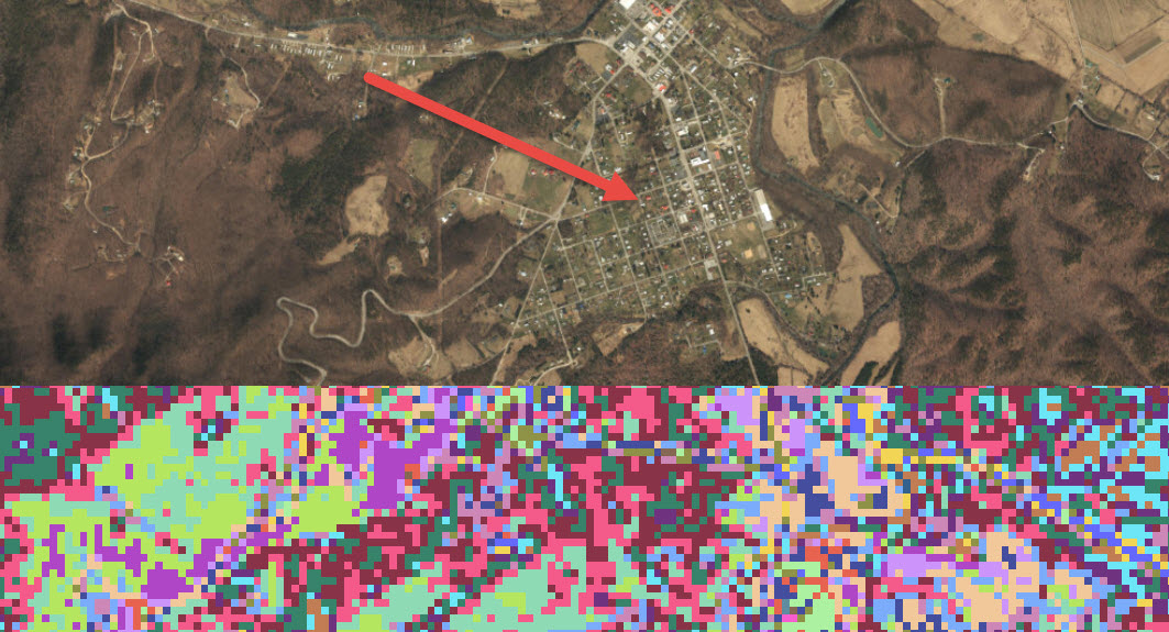
Figure 21.22. Associating urban areas with red

Some questions—should golf courses be classified as agriculture or urban, or should you create a new category? The same decisions must be made for all classes, including the extensive tree canopy coverage in an urban area—should that be classified as urban or forest? We have only four informational classes to choose from.

Since we only used the 25 classed image, the golf course spectral cluster fell into multiple spectral clusters—agriculture, forest, and urban—except for a water hazard (Figure 21.23). We are only using the 25 spectral classes; this image should have at least 50 to classify it more accurately.

Using unsupervised classification with this image, was it easy to identify clouds? For purposes of this exercise, clouds were placed into their own class. How about cloud shadows? What were cloud shadows classified? Again, increasing the number of spectral clusters would have enabled us to provide more definitive land cover class assignments.

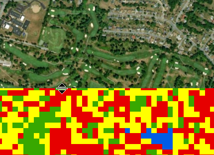
Figure 21.23 Golf course classified into multiple categories

After assigning all 25 spectral classes, look at the overall image (Figure 21.24). Are the informational classes generally correct? Do you have any blue areas within the mountains that are not water? Urban classes, that are in the water? For our image, the answer is yes to all of these questions, which again tells us that 25 spectral clusters were insufficient to separate all of the spectral clusters so we could categorize them into information classes.

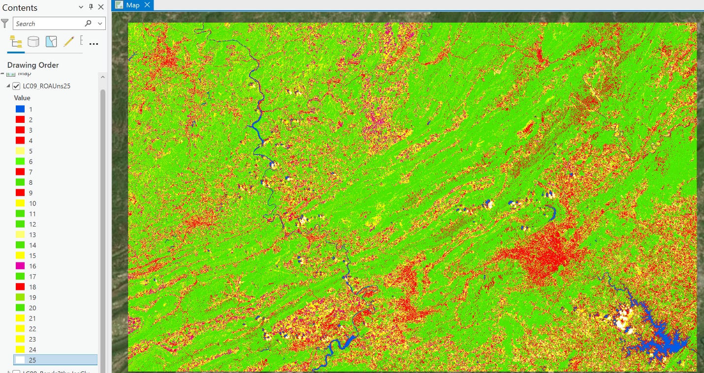
Figure 21.24. Spectral clusters assigned to four colors

We are not yet finished because, in Contents, the symbology lists 25 spectral values but only four colors that pertain to our informational classes (five colors if you have included a separate class for clouds).

Continue to spot-check the results. Doing a complete accuracy assessment of all categories at this juncture is unnecessary. An accuracy assessment, the final step required in any image classification scheme, will be covered in the last chapter of this book—Chapter 25: Accuracy Assessment. We will now demonstrate how to assign spectral classes to informational classes.

Reclassifying Spectral Classes into Informational Classes

The 25 spectral classes have been assigned the colors of the four informational classes. To change this to four informational classes, open the Geoprocessing pane (select the Analysis tab on the ribbon and Tools) and search for Reclass. Choose Reclassify (Spatial Analyst Tools) (Figure 21.25).

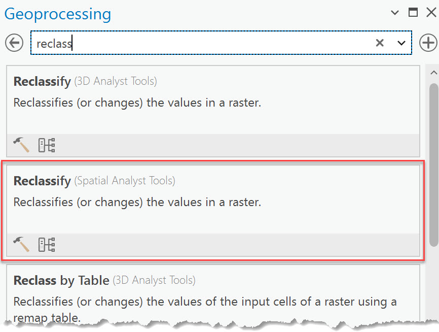
Figure 21.25. The Reclassify tool

The Input raster is the Unsupervised 25 layer we have been working with. Once that layer is selected, the Reclassification table expands and lists all 25 values under the Value and New columns. Use the symbology of the Unsupervised 25 layer as a guide. Figure 21.26

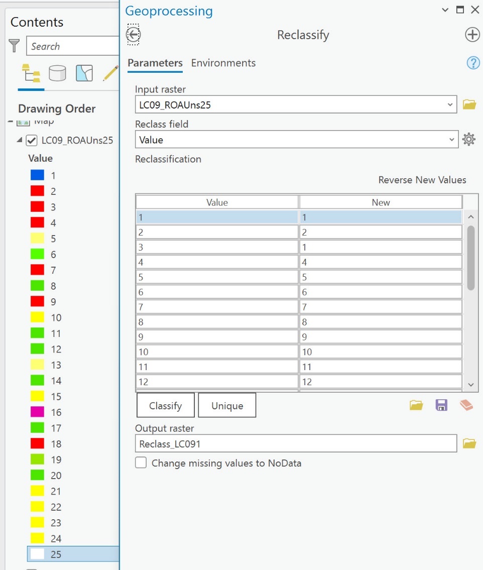
Figure 21.26. The reclassification table

• All values coded as Red are Urban/built up/transportation; change to 1 in the New column
• All values coded as Yellow are Mixed Agriculture; change to 2 in the New column
• All values coded as Green are Forest & Wetland; change to 3 in the New column
• All values coded as Blue are Open water; change to 4 in the New column

Click in the row under New and make the change. Do this line by line for all 25 Values (Figure 21.27). Don’t miss any! Be sure you name the Output raster something you will understand.

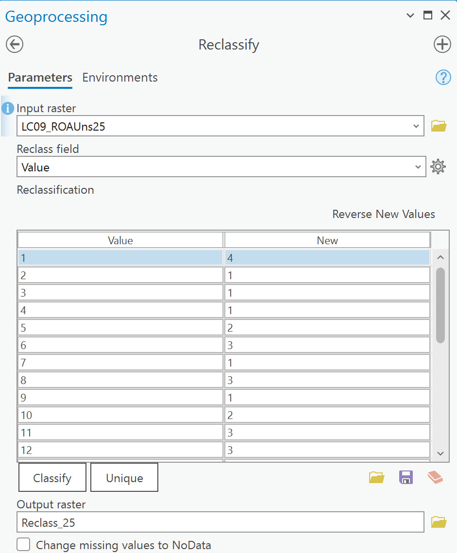
Figure 21.27. The Reclassify tool

Click Run.

Once finished, the new layer will appear in Contents, with the new image in the map viewer. The colors seen may differ from those in Figure 21.28, as these are randomly assigned, and we must assign the correct colors.

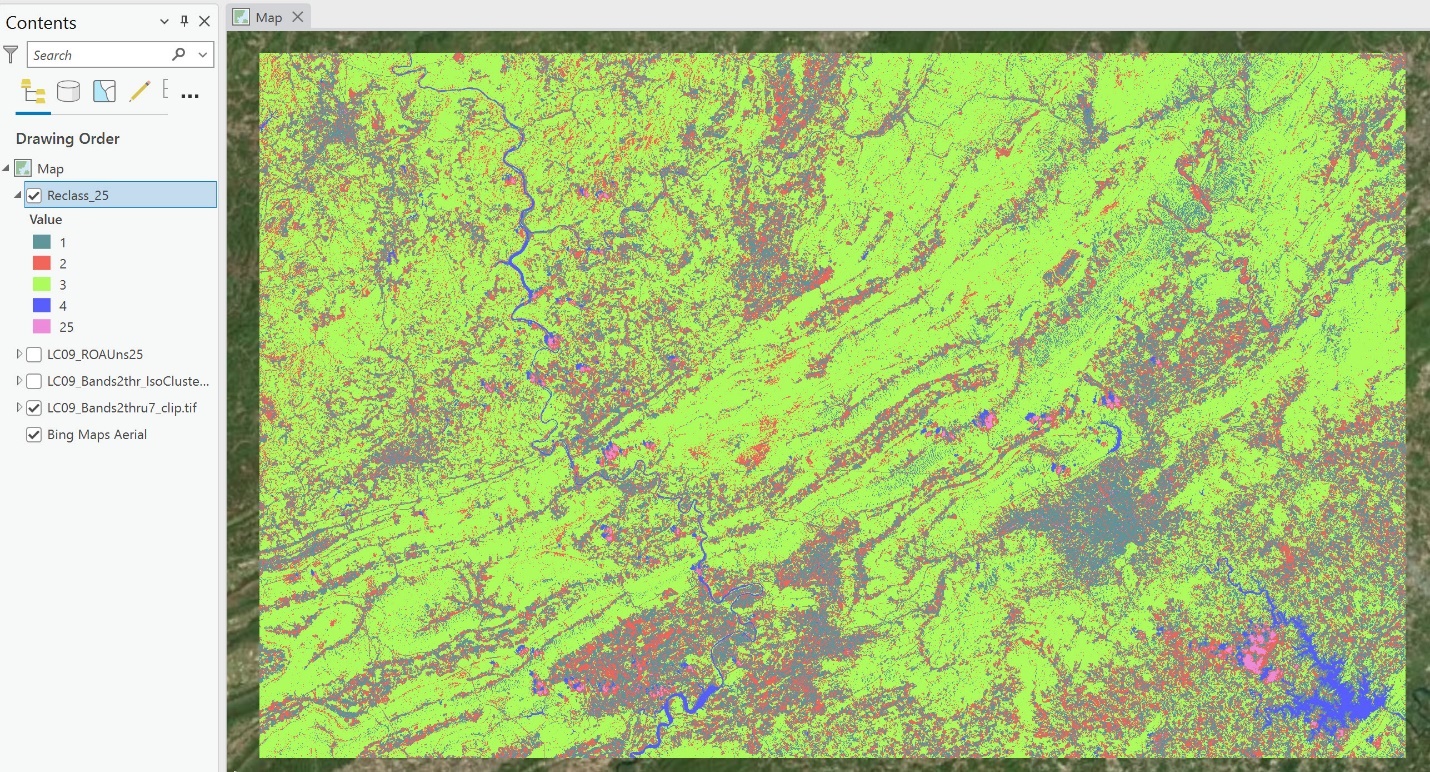
Figure 21.28. A reclassified image

Go to symbology and change the color scheme. Under the Label column, type the informational class name on the row associated with its designated color (Figure 21.29).

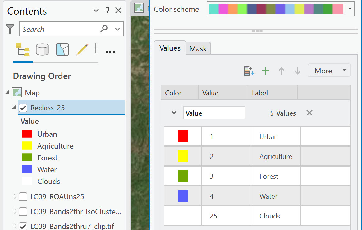
Figure 21.29. Reassigning colors to the new image

The two images, the spectral class image with the 25 values and the informational class image with four values, should look the same if the Reclass process was completed correctly (Compare Figure 21.24 with Figure 21.29).

Calculating the Percent of Total Area for Each Informational Class

Once the pixels have been reclassified into four classes, the percentage of the total area for each class can be easily calculated. To do this, right-click the Reclass raster and open the Attribute Table. This table provides the number of cells, Count, in each informational class (Figure 21.30).

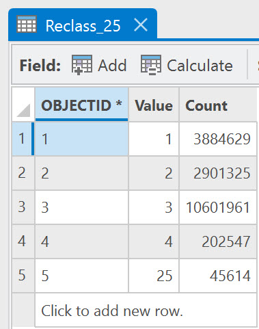
Figure 21.30. The attribute table

The percentage of the total area for each informational class can be calculated within the Attribute Table. First, select Add to add a field (Figure 21.31).

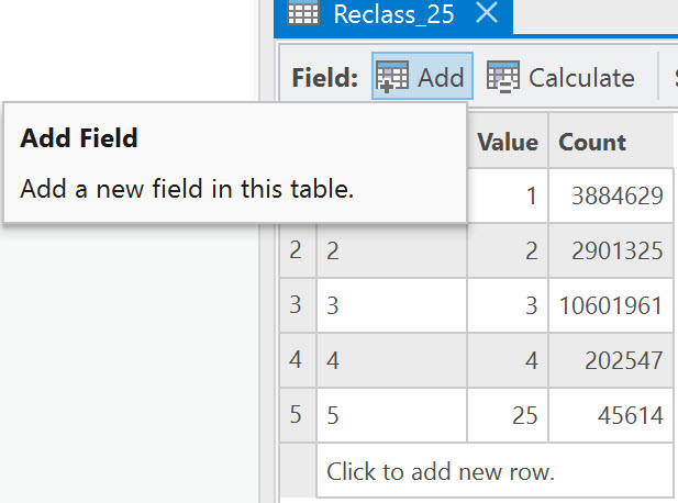
Figure 21.31. The attribute table

Then name the field, percent, and tab to each column to choose the parameters. Under Data type, choose Float (the number will be a real number). Under Number Format, choose Numeric. For the options under Numeric, 2 Decimal places should be sufficient for a percentage. Add a second field for Hectares. (Figure 21.32)

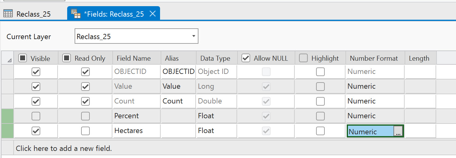
Figure 21.32. Adding a field to the attribute table

To save the new field, click Save in the Fields tab on the ribbon (Figure 21.33). Then close the Fields: Reclass25 tab at the top of the attribute table.

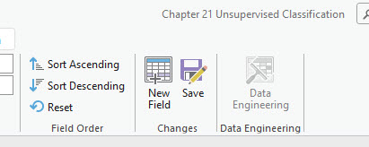
Figure 21.33. Saving the changes to the attribute table

We first need to know how many pixels are in the entire image to calculate the percentage for each informational class. Since we only have four categories (actually five categories including clouds), add them together (answer = 17,636,076). Is this correct? Check the number of rows and columns under Properties (3294 x 5354 = 17,636,076). Please note that your total may differ as you may not have the same subset displayed here.

To calculate the value for the field, right-click the new field in the attribute table and select Calculate Field (Figure 21.34).

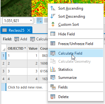
Figure 21.34. Calculating the new field

In the Calculate Field dialog box, you will complete the Expression for Percent = (Figure 21.35).

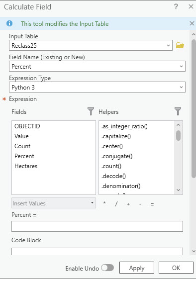
Figure 21.35. Calculating the new field

As shown in Figure 21.36, enter the expression under Percent= exactly as follows, except for the total cell count—your number will likely differ.

(!Count! / 8881691) * 100

Click OK.

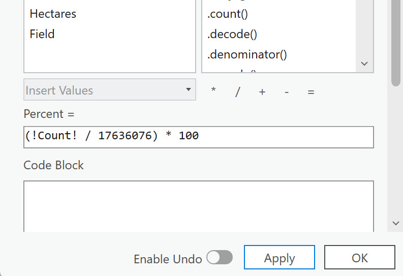
Figure 21.36. Calculating the new field

The new field now shows the percentage of the total for each informational class (Figure 21.37).

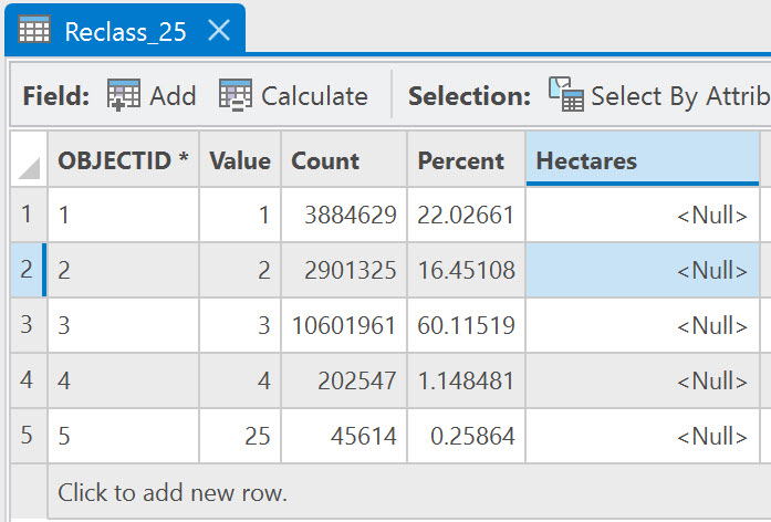
Figure 21.37. Calculating the new field

Now calculate the hectare field; the formula is (!Count! *900) / 10000 (Figure 21.38).

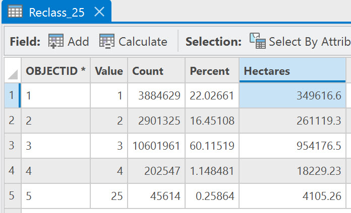
Figure 21.38. Calculating the new field

Before we finish up, let’s discuss one option under the ISO Cluster Unsupervised Classification Geoprocessing tool that we did not use—Output signature file (Figure 21.39).

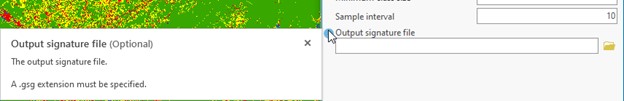
Figure 21.39. Saving the signature file

We did not create this during our geoprocessing operation. Entering a name here and saving a signature file generates multivariate statistics for each cluster. The signature file can be read using any text editor, such as Microsoft Notepad. The statistics generated are related to the spectral values, not the informational categories. They can be used to evaluate co-variance between any of the bands within your multispectral image. 

How accurate was the ISO Cluster Unsupervised Classification method and 25 classes? That is assessed in the last chapter of this book—Chapter 25: Accuracy Assessment. You may proceed directly to that chapter. But we recommend you complete Chapters 22 – 24, covering the supervised classification process.