16 Gas Transport
Learning objectives
- Describe how the affinity of hemoglobin for oxygen changes from the normal lung to metabolizing tissue and the local factors that contribute to these changes.
- Compare and contrast the following three terms: oxygen partial pressure, oxygen saturation, and oxygen content.
- Describe the three modes of transport of carbon dioxide by blood.
Oxygen Transport
Because of its relative lack of solubility, the transport of oxygen must involve a protein carrier, which is of course hemoglobin. In this chapter we will look at the characteristics of hemoglobin that make it an ideal and rather sophisticated carrier molecule, capable of not only picking up oxygen at the lungs, but just as importantly dropping it off at the tissue. Before that, let us briefly look at its structure (but leave most of the details to the biochemists).
The hemoglobin molecule consists of four polypeptide chains, two alpha and two beta (figure 16.1). These proteins comprise the “globin” part of the molecule but are not simply structural as they contain sites that are capable of receiving CO2 and also hydrogen ions—a handy function, as you might imagine. Some anemias, such as sickle cell anemia, involve a conformational change in these proteins and diminish the molecule’s gas carrying ability.
![a. Hemoglobin - 4 distinct subunits labeled α1, α2, β1, and β2. All contain a circle representing the iron-containing heme group in their center. b. Iron-containing heme group - IUPAC name 3-[18-(2-carboxyethyl)-7,12-bis(ethenyl)-3,8,13,17-tetramethyl porphyrin-21,23-diid-2-yl]propanoic acid;iron(2+)](https://pressbooks.lib.vt.edu/app/uploads/sites/73/2022/05/16.1.png)
The heme component of hemoglobin is an iron-containing porphyrin molecule capable of binding with oxygen. Each of the four polypeptide chains contains a heme molecule, meaning that each hemoglobin molecule is capable of transporting four oxygen molecules. It is also worth noting that binding of oxygen to the heme molecule induces a conformational change that results in oxyhemoglobin having some different behaviors and indeed color to deoxyhemoglobin. We will look at some of these differences in behavior later on.
It is also worth reviewing hemoglobin’s home here as well—the red blood cell (RBC). The red blood cell’s classic biconcave shape provides a large surface area for gas exchange and also means that no hemoglobin molecule inside is very far from the edge of the cell, cutting down on the diffusion distance of gases. The cell is also very flexible, making it capable of squeezing through narrow and twisting capillaries so that its walls and those of the capillary may be in close contact and again diffusion distances are reduced.
Each RBC is capable of holding up to 250 million hemoglobin molecules, so consequently is capable of holding one billion oxygen molecules; as such the RBC fulfills its primary role of oxygen transport well. This oxygen transport system fails in anemias that result in either too few red blood cells or too little hemoglobin in each cell (or both). Now let us look at the behavior of hemoglobin.
The behavior of hemoglobin is best described by the oxygen saturation curve (figure 16.2), and this is one of the most important curves to understand in medicine. The curve shows the percentage of hemoglobin that has all of its heme molecules bound with oxygen (i.e., are saturated). So for example a 50 percent saturation would mean that half of the heme sites were occupied by oxygen. The curve shows percentage saturation in relation to oxygen partial pressure, and what should be immediately noticeable is that the higher the partial pressure of oxygen then the greater the saturation. But the relationship is far from linear and its shape offers several important physiological advantages. If it helps understand it, think of this curve as an instruction manual for hemoglobin, telling how saturated it should be at any PO2. In reality it is an enzyme kinetics curve, describing hemoglobin’s affinity for oxygen over a range of PO2.
First let us put the curve in a physiological context. The alveolar PO2 is around 100 mmHg. This means that as blood passes the alveoli and is exposed to this PO2, then oxygen saturation becomes close to 100 percent, about 98 percent. The first important physiological feature of this curve is that PO2 can fall a considerably long way before it has an impact on oxygen saturation. So, taking time to look at the numbers on the graph, let us say, for example, that a patient begins to hypoventilate and alveolar PO2 falls to 70 mmHg; while this is a considerable fall in PO2, the saturation will only fall a few percentage points, and PO2 must fall to 50 before significant loss of saturation, or desaturation, occurs. Below 50, however, notice how the curve rapidly steepens, and now for a small change in PO2, we get a large desaturation.
This steep section of the curve is therefore clinically critical. If your patient’s saturation monitor reads 83 percent what should spring into your mind is it that such a low saturation puts the patient onto the steep part of the curve. It will now take only a small further decline in alveolar PO2 to have a profound effect on saturation, unlike at the top and flat section of the curve where small changes in alveolar PO2 have very little effect on saturation.
So what is the advantage of having such a steep curve at lower PO2s? Let us look at the physiological situation again. We have already said that the alveolar PO2 of 100 results in a saturation close to 100 percent (i.e., at the lung the hemoglobin has a high affinity for oxygen and becomes fully saturated).
At the tissue, however, we want hemoglobin to lose its affinity for oxygen and release some to the metabolizing cells. At the tissue the local PO2 is much lower, around 40, because of the oxygen consumption by the tissue. At the lower PO2, hemoglobin’s affinity for oxygen falls, and it will lose some of its oxygen to the tissue and saturation will fall. This is ideal, as now our oxygen carrier is capable of releasing oxygen where it is needed.
If tissue PO2 falls even lower, such as when metabolic rate is high, then more oxygen will be released by hemoglobin as its affinity for oxygen declines with the lower tissue PO2. Therefore the delivery system for oxygen is intrinsically tied to metabolic rate.
The shape of this curve makes hemoglobin a remarkable molecule—able to grab oxygen at the oxygen-providing lung, but relinquish it to oxygen-demanding tissue and relinquish more when the tissue needs more. There are other factors that fine-tune the amount of oxygen delivered to tissue to match its oxygen demand. This is summarized in figure 16.3.
Shifts in the O2 Saturation Curve
The metabolic rate of tissue determines its oxygen demand, with more active tissue requiring hemoglobin to relinquish more oxygen. So there are several other factors, beyond low local PO2, that are associated with active tissue that cause hemoglobin to reduce its affinity for oxygen and therefore release it. Tissue with a high metabolic rate tends to have (1) higher temperature, (2) high PCO2, and (3) lower pH. We can look at the effect of each of these factors on the saturation curve.
Shifts with temperature: Figure 16.4 shows the saturation curve at difference tissue temperatures. The curve we have just looked at was at 38ºC. Notice that as temperature is reduced, the curve shifts to the left, but more importantly (physiologically) when temperature increases then the curve shifts to the right. Let us look at what this means in terms of hemoglobin’s affinity for oxygen (follow the numbers on the graph again). As before, we will assume that our tissue PO2 is 40 mmHg, and at normal temperatures this results in a saturation of about 70 percent.
Now at the same PO2 but a higher temperature (e.g., 43ºC) the hemoglobin O2 saturation falls to a little over 50 percent, meaning that more oxygen has been relinquished to the tissue (i.e., an increase in temperature reduces hemoglobin’s affinity for oxygen).
Shifts with CO2: We see a similar situation with a rise in PCO2, shown in figure 16.5 with the saturation curve at different PCO2s. At a normal arterial PCO2 (40 mmHg) we get the same saturation curve that we saw previously. But if PCO2 is raised, such as in the locality of highly active tissue (e.g., 80 mmHg), then the curve shifts rightward. Again this means that hemoglobin’s affinity is lowered at equivalent PO2 and more oxygen is released, resulting in a lower saturation.
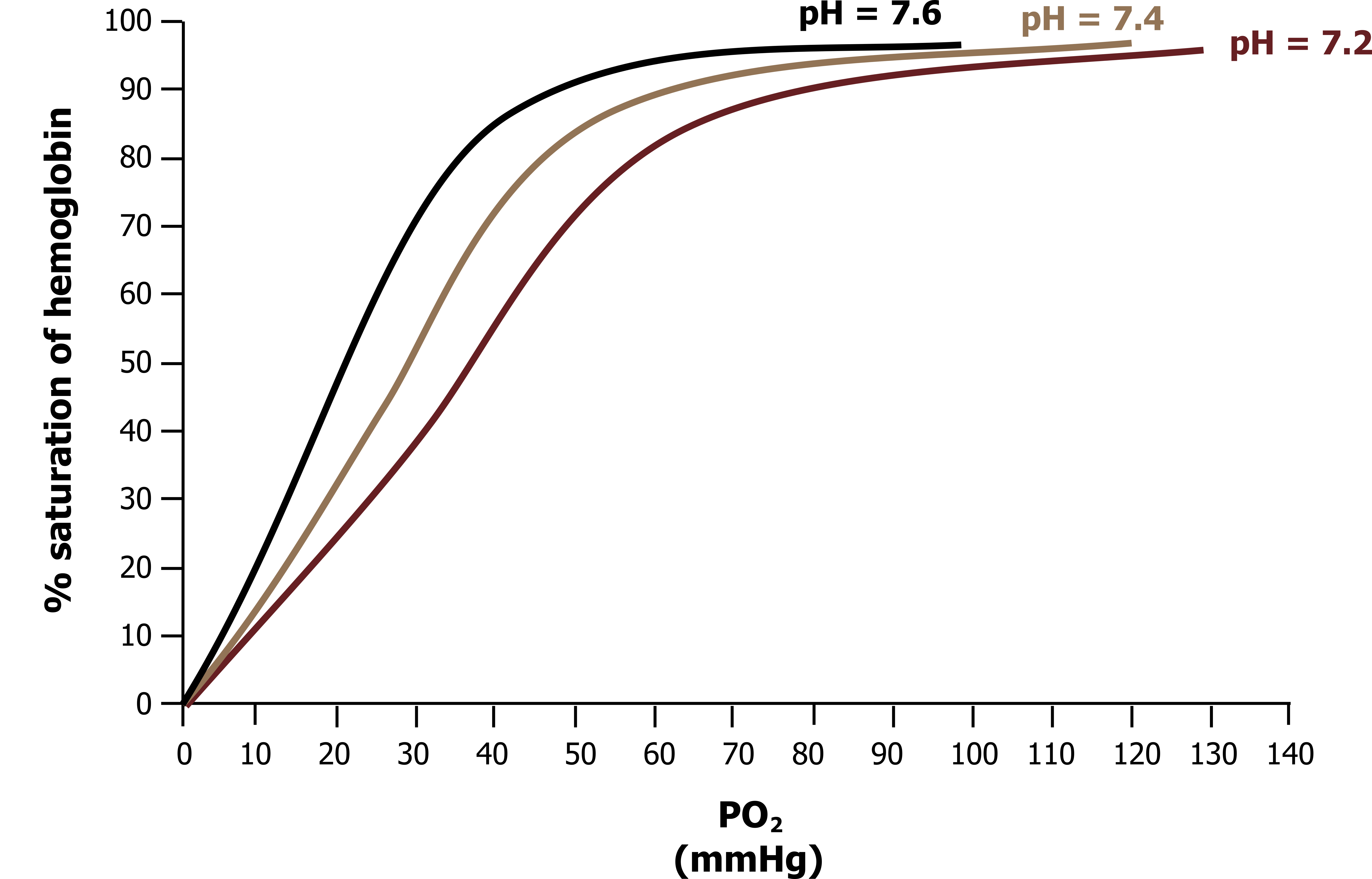
Shifts with pH: Finally, the same is true for changes in pH, shown in figure 16.6 with the curve at different pHs. When pH falls, as in active tissue, then the curve shifts rightward from its normal position at normal pH (7.4). Again, this result describes a lowered affinity for oxygen, so at equivalent levels of PO2 more oxygen is released when the hemoglobin enters a low pH environment (e.g., 7.2 shown on figure 16.6). Obviously pH and PCO2 are related, and their effect on hemoglobin binding is known as the Bohr effect.
One last factor that causes this rightward shift is 2,3 diphosphoglycerate, or DPG. DPG is an end product of RBC metabolism, and as it increases inside the cell it reduces hemoglobins, affinity for oxygen. Elevated DPG levels are associated with chronic hypoxia, such as experienced at altitude or more pertinently in the presence of chronic lung disease. Conversely, DPG levels are lower in stored blood, so transfused blood may have a problem giving up its oxygen.
All these factors mean that hemoglobin will deliver more oxygen to busy tissue.
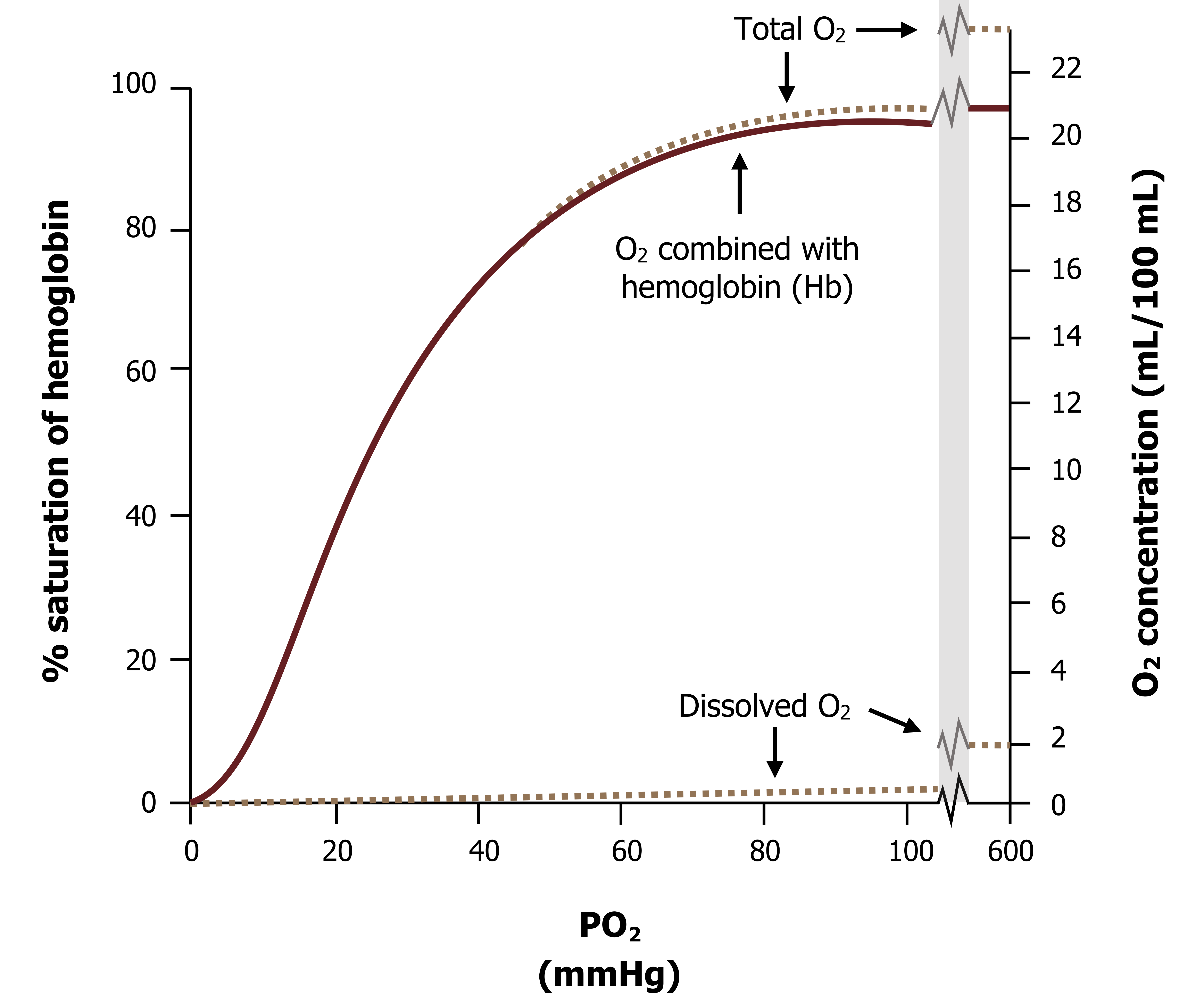
Total oxygen carriage: So far we have discussed oxygen transport in terms of hemoglobin only. But despite its lack of solubility, some oxygen can dissolve into the plasma. Realistically this is a very small amount at physiological partial pressures (i.e. at an alveolar PO2 of 100 mmHg only a fraction of a milliliter of oxygen will dissolve into the blood, as figure 16.7 shows).
Obviously this amount of oxygen is completely inadequate to support metabolism and illustrates the need for hemoglobin. But this minute amount when added to the O2 combined to the hemoglobin makes up the total O2 content of the blood. When calculating the oxygen content of the blood we must consider both of these compartments—hemoglobin and plasma (figure 16.8).

Calculating the O2 Content of Blood
To calculate the arterial oxygen content (CaO2) let us first look at the factors affecting the majority of the O2 (i.e., that carried by hemoglobin).
(1) This will be determined by the amount of hemoglobin in the blood (measured in mg/dL). So let us start building the equation.
Equation 16.1
[latex]C_aO_2 = Hb (mg/dL)...[/latex]
(2) Second, we must consider the oxygen carrying capacity of Hb, which is 1.34 mL O2/gm Hb. So we multiply the amount of Hb by its carrying capacity.
Equation 16.2
[latex]C_aO_2 = Hb (mg/dL) \times 1.34\, O_2/gmHb...[/latex]
(3) But that carrying capacity might not have been reached by all the Hb (i.e., the Hb may not be fully saturated). So to account for this, we multiply by the saturation (SaO2).
Equation 16.3
[latex]C_aO_2 = Hb (mg/dL) \times 1.34\, O_2/gmHb \times S_aO_2...[/latex]
(4) So far that takes care of the O2 associated with Hb (normally about 98 percent of the total). Now we must add the O2 in plasma to the equation. We do this by measuring the PaO2 and multiplying it by a solubility coefficient (0.003 mL O2/mmHg/dL) to convert it from a partial pressure to milliliters. Removing the units makes this long but simple equation a little easier to understand. It has two components, representing the two compartments for O2 carriage.
Equation 16.4
[latex]C_aO_2 = (Hb \times 1.34 \times S_aO_2) + (P_aO_2 \times 0.003)[/latex]
The plasma component is usually inconsequential, but may become more important when blood is exposed to an elevated alveolar PO2, such as during oxygen or hyperbaric therapy.
Summary
So to summarize, as oxygen’s lack of solubility means metabolic demands cannot be met by dissolved oxygen alone, the vast majority of oxygen is transported by hemoglobin, a molecule that is beautifully designed to pick up oxygen at the lung and release oxygen in proportion to the tissue’s demand. We will see more of hemoglobin’s sophistication when we address CO2 carriage.
CO2 Transport
Unlike oxygen, carbon dioxide is soluble enough that it does not need a protein carrier like oxygen needs hemoglobin to enter and exit plasma. However, this does not necessarily mean that CO2 transport is simple. The complication this time is that free dissolved CO2 forms carbonic acid, which can threaten pH homeostasis. So most CO2 is not transported in the dissolved form. Most (approximately 70 percent) of the CO2 that emerges from metabolizing tissue is converted to bicarbonate with the help of enzymes within red blood cells. We will look at this more closely in a moment. About 15–25 percent is transported on hemoglobin.
Transport on Hemoglobin (15–25 Percent)
Carbon dioxide can bind to the terminal amine groups of hemoglobin’s polypeptide chains forming carbaminohemoglobin. It is worth noting a couple of points about this. First, CO2 does not compete with oxygen to bind to Hb—the binding sites are completely different and hemoglobin can hold both CO2 and O2 at the same time. Second, deoxyhemoglobin is a better carrier of CO2 than oxyhemoglobin is; consequently at the tissue where hemoglobin is losing its oxygen it is becoming a more efficient CO2 transporter. This is known as the Haldane effect.
Transport as Dissolved CO2 (About 7 Percent)
A little CO2 combines with water to produce carbonic acid, the dissociated hydrogen form that must be buffered by plasma proteins, such as albumin.
Transport as Bicarbonate (About 70 Percent)
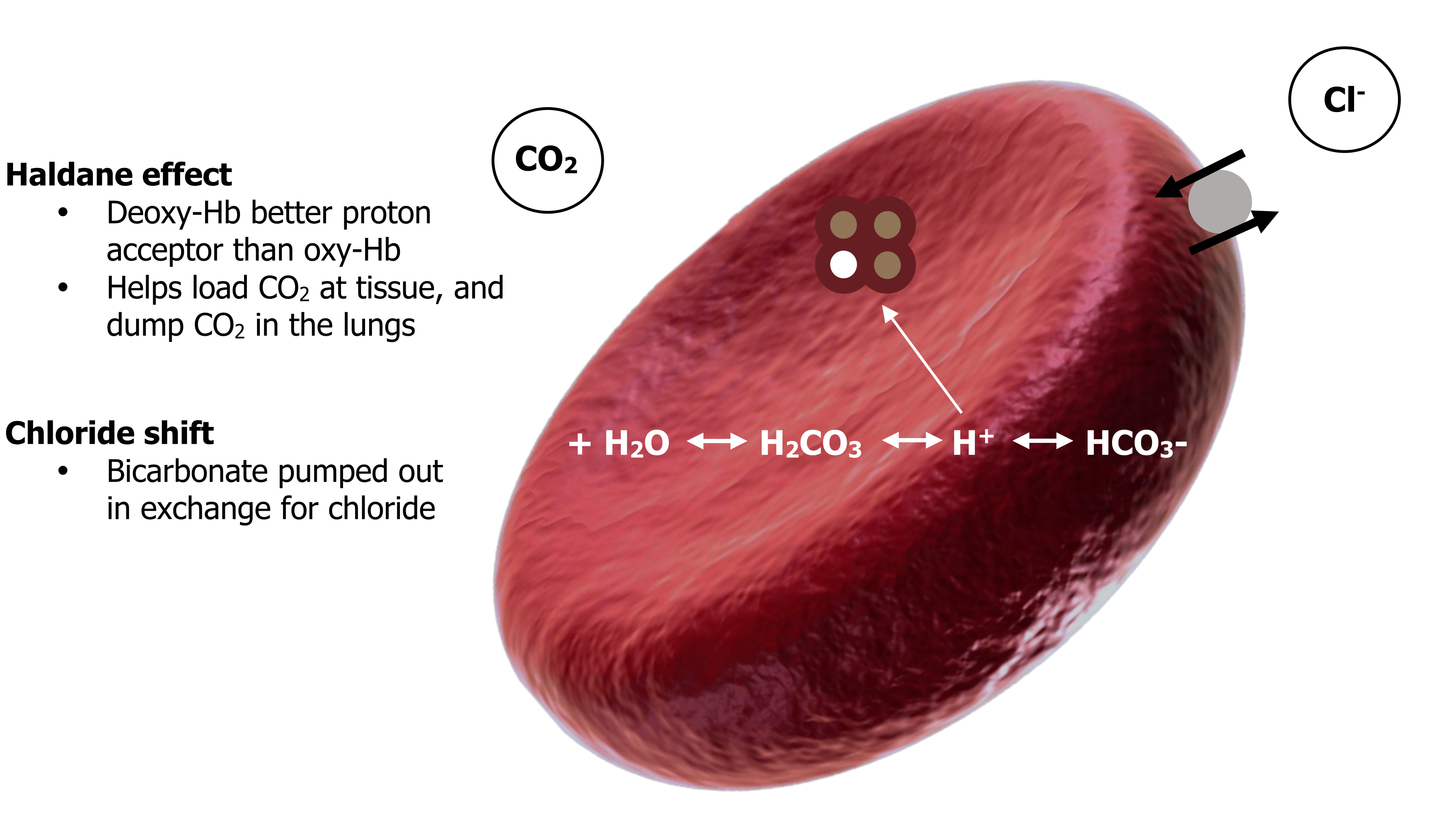
Seventy percent of the CO2 enters red blood cells, and once inside a familiar reaction occurs (equation 16.5). The CO2 binds with water in the cytoplasm, producing carbonic acid, which then dissociates into a hydrogen ion and a bicarbonate ion.
This reversible reaction is accelerated by the enzyme carbonic anhydrase and is driven rapidly to the right by the high concentration of CO2 at the tissue.
The hydrogen ion produced helps shift the oxygen saturation curve to the right and so promotes further release of oxygen to the tissue. Hemoglobin then serves yet another purpose by buffering the proton with its polypeptide chains. Deoxyhemoglobin is a better proton acceptor than oxyhemoglobin, so as the hemoglobin loses its oxygen at the tissue it becomes a better pH buffer. This reduces the amount of hydrogen ion on the right side of our equation and moves the equation to the right, promoting the conversion of more CO2.
Equation 16.5
[latex]CO_2 + H_2O \leftrightarrow H_2CO_3 \leftrightarrow H^+ + HCO_3-[/latex]
High concentrations of CO2 at the tissue push this equation right to produce bicarbonate.
The bicarbonate ion is pumped out of the cell, but without intervention this would leave the inside of the cell too positively charged as the negative charge of the bicarbonate is lost. To maintain electroneutrality the bicarbonate is exchanged for a chloride ion; this process is referred to as the chloride shift. The formation of bicarbonate at the tissue is summarized in figure 16.9.
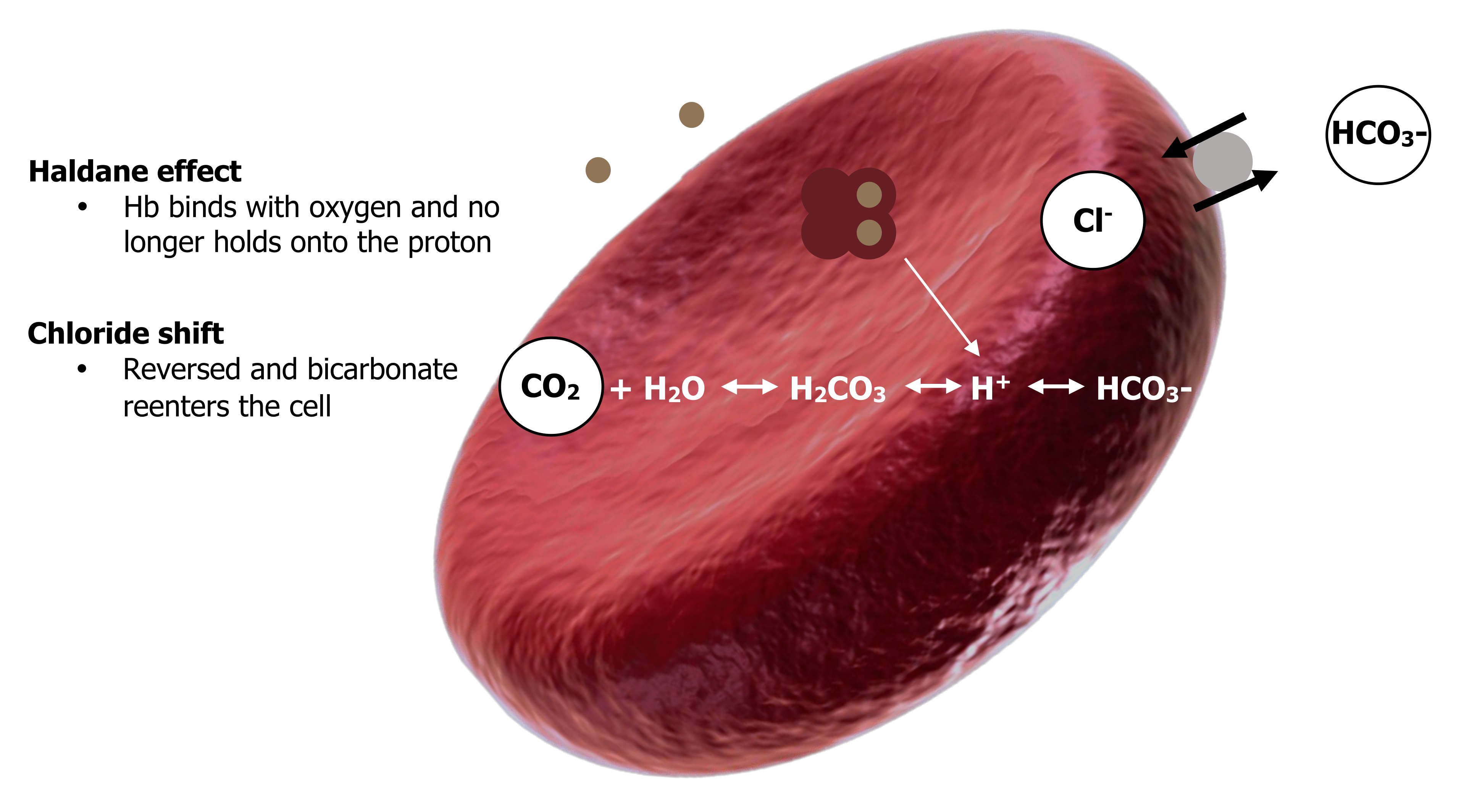
The CO2 now travels through the bloodstream as bicarbonate toward the lungs. At the lungs the process is basically reversed. The partial pressure of CO2 at the lungs is low; consequently our equation is driven toward the left-hand side as CO2 leaves toward the low alveolar PCO2 (equation 16.6).
Equation 16.6
[latex]CO_2 + H_2O \leftrightarrow H_2CO_3 \leftrightarrow H^+ + HCO_3-[/latex]
←
High bicarbonate and low CO2 at the lung force the equation leftward.
The high alveolar PO2 also promotes the leftward movement—binding of oxygen to hemoglobin makes hemoglobin a less effective proton binder so it loses the proton and raises the amount of substrate on the right-hand side and thereby promotes reformation of CO2. The Haldane effect is also reversed—as hemoglobin gains oxygen at the lung it loses its affinity for CO2 and releases it into the plasma. This raises plasma PCO2 and promotes diffusion of CO2 into the alveoli for expulsion.
Likewise the chloride shift is reversed and bicarbonate reenters the cell as chloride is pumped back out.
All these moves help promote the right-to-left direction of our now infamous equation and the re-forming of CO2. Alveolar ventilation gets rid of the re-formed CO2 to the atmosphere, maintaining the alveolar PCO2 at relatively low levels and the direction of the equation right-to-left. The reformation of CO2 at the lungs is summarized in figure 16.10.
The CO2 “Dissociation” Curve
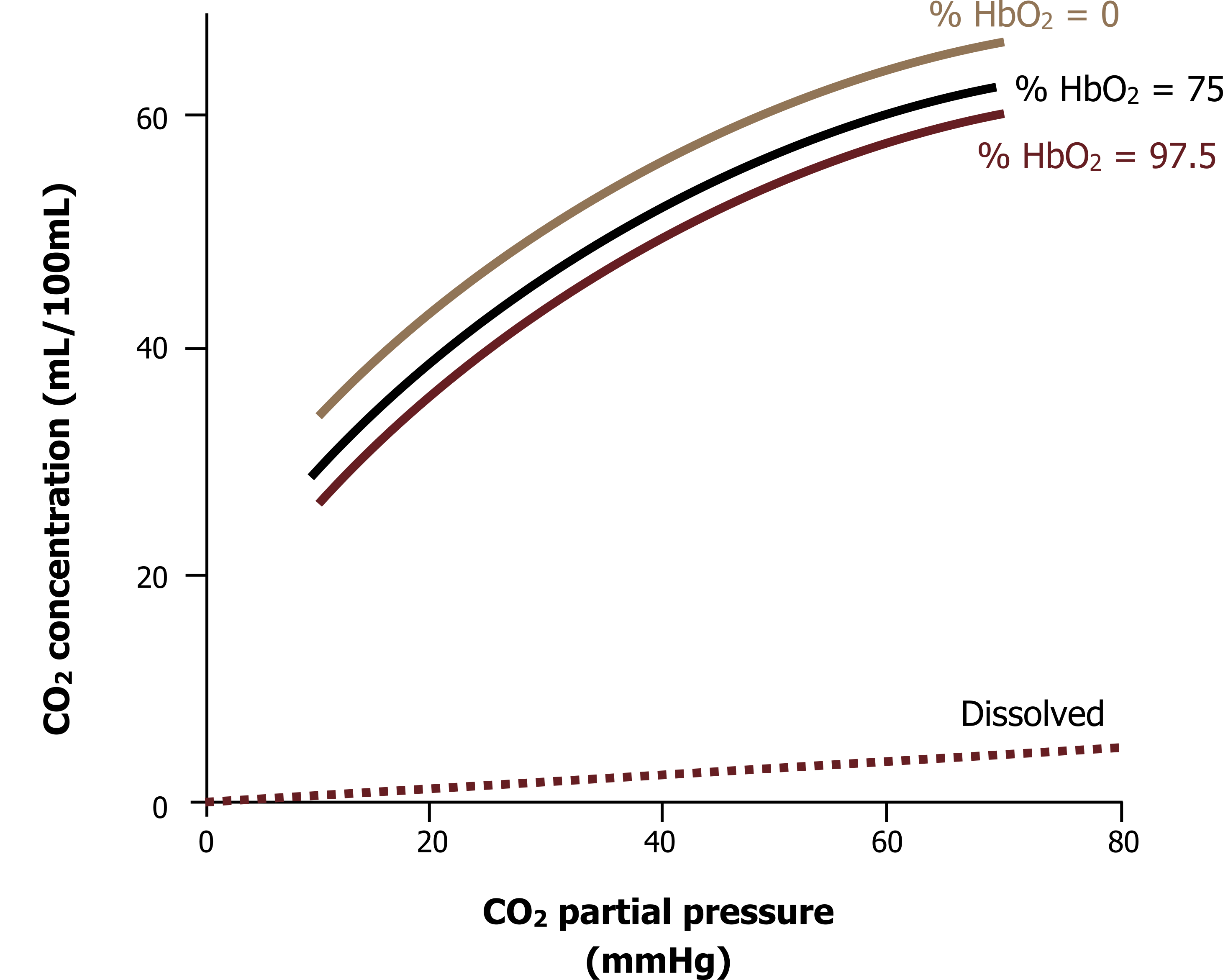
So, for want of a better name, we can also draw a CO2 dissociation or saturation curve, as is shown in figure 16.11. The graph shows the CO2 concentration in blood across a wide range of PCO2 and shows the effect of Hb O2 saturation on CO2 carriage. The CO2 dissociation curve is unlike the oxygen saturation curve and is virtually linear (i.e., the higher the PCO2, the higher the CO2 content of the blood); there is no plateau to the curve as we saw with O2 transport. The ramification of this is that the lower the alveolar PCO2, the lower the blood PCO2, and the higher the alveolar PCO2, the higher the blood PCO2. It is a very simple relationship that ends with the obvious statement that the more you breathe, the lower arterial CO2 becomes. It is worth reminding ourselves here that this is not a relationship seen with oxygen that is limited by the capacity of hemoglobin (breathing more does not necessarily result in more oxygen in the bloodstream). The other aspect to note here is the effect of hemoglobin’s oxygen saturation on carbon dioxide carriage. This has clinical ramifications, so we will look at this more closely.
When deoxygenated, hemoglobin’s structure promotes binding of CO2 and buffering of protons by the polypeptide chains. So when O2 saturation is zero, the CO2 and proton carrying capability of Hb is high. As already mentioned, this means that when Hb is in its deoxygenated form at the tissue, its CO2 carrying ability is increased.
When we get to the lung, however, the Hb is exposed to the high alveolar PO2 and oxygen binds to the heme sites and becomes saturated; this causes a conformational change, and the CO2 and proton carrying ability is reduced. So conveniently CO2 release is promoted at the lung.
Summary
Although CO2 is highly soluble, very little of it can be transported as dissolved CO2 in plasma because of its effect on pH. The majority is converted to bicarbonate in red blood cells and transported in plasma, while about 25 percent is transported bound to hemoglobin.
References, Resources, and Further Reading
Text
Levitsky, Michael G. “Chapter 7: Transport of Oxygen and Carbon Dioxide in the Blood.” In Pulmonary Physiology, 9th ed. New York: McGraw Hill Education, 2018.
West, John B. “Chapter 6: Gas Transport by the Blood—How Gases Are Moved to the Peripheral Tissues.” In Respiratory Physiology: The Essentials, 9th ed. Philadelphia: Wolters Kluwer Health/Lippincott Williams and Wilkins, 2012.
Widdicombe, John G., and Andrew S. Davis. “Chapter 6.” In Respiratory Physiology. Baltimore: University Park Press, 1983.
Figures
Figure 16.1: Basic structure of hemoglobin. OpenStax College. 2013. CC BY 3.0. https://commons.wikimedia.org/wiki/File:1904_Hemoglobin.jpg [added polypeptide chain]
Figure 16.2: Hemoglobin saturation curve. Grey, Kindred. 2022. CC BY 4.0. https://archive.org/details/16.2_20220125
Figure 16.3: The hemoglobin saturation curve. Grey, Kindred. 2022. CC BY 4.0. https://archive.org/details/15.1-needs-numbering
Figure 16.4: Effect of temperature on the saturation curve. Grey, Kindred. 2022. CC BY 4.0. https://archive.org/details/16.4_20220125
Figure 16.5: Effect of PCO2 on the saturation curve. Grey, Kindred. 2022. CC BY 4.0. https://archive.org/details/16.5_20220125
Figure 16.6: Effect of pH on the saturation curve. Grey, Kindred. 2022. CC BY 4.0. https://archive.org/details/16.6_20220125
Figure 16.7: Oxygen carriage. Grey, Kindred. 2022. CC BY 4.0. https://archive.org/details/16.7_20220125
Figure 16.8: Compartment of blood oxygen content. Grey, Kindred. 2022. CC BY 4.0. https://archive.org/details/16.8_20220125
Figure 16.9: Formation of bicarbonate at the tissue. Grey, Kindred. 2022. CC BY-SA 3.0. Added Erythrocyte deoxy by Rogeriopfm from WikimediaCommons [added text around image]. CC BY-SA 3.0. https://archive.org/details/15.2-needs-numbering
Figure 16.10: Reformation of CO2 at the lungs. Grey, Kindred. 2022. CC BY-SA 3.0. Added Erythrocyte deoxy by Rogeriopfm from WikimediaCommons [added text around image]. CC BY-SA 3.0. https://archive.org/details/15.3
Figure 16.11: CO2 dissociation curve. Grey, Kindred. 2022. CC BY 4.0. https://archive.org/details/15.4_20220125
