9 Crustal Deformation and Earthquakes
Learning Objectives
By the end of this chapter, students should be able to:
- Differentiate between stress and strain.
- Identify the three major types of stress.
- Differentiate between brittle, ductile, and elastic deformation.
- Describe the geological map symbol used for strike and dip of strata.
- Name and describe different fold types.
- Differentiate the three major fault types and describe their associated movements.
- Explain how elastic rebound relates to earthquakes.
- Describe different seismic wave types and how they are measured.
- Explain how humans can induce seismicity.
- Describe how seismographs work to record earthquake waves.
- From seismograph records, locate the epicenter of an earthquake.
- Explain the difference between earthquake magnitude and intensity.
- List earthquake factors that determine ground shaking and destruction.
- Identify secondary earthquake hazards.
- Describe notable historical earthquakes.
Crustal deformation occurs when applied forces exceed the internal strength of rocks, physically changing their shapes. These forces are called stress, and the physical changes they create are called strain. Forces involved in tectonic processes as well as gravity and igneous pluton emplacement produce strains in rocks that include folds, fractures, and faults. When rock experiences large amounts of shear stress and breaks with rapid, brittle deformation, energy is released in the form of seismic waves, commonly known as an earthquake.
9.1 Stress and Strain
Stress is the force exerted per unit area and strain is the physical change that results in response to that force. When applied stress is greater than the internal strength of rock, strain results in the form of deformation of the rock caused by the stress. Strain in rocks can be represented as a change in rock volume and/or rock shape, as well as fracturing the rock. There are three types of stress: tensional, compressional, and shear. Tensional stress involves forces pulling in opposite directions, which results in strain that stretches and thins rock. Compressional stress involves forces pushing together, and compressional strain shows up as rock folding and thickening. Shear stress involves transverse forces; the strain shows up as opposing blocks or regions of material moving past each other.
| Type of stress | Associated plate boundary type (see chapter 2) | Resulting strain | Associated fault and offset types |
|---|---|---|---|
| Tensional | Divergent | Stretching and thinning | Normal |
| Compressional | Convergent | Shortening and thickening | Reverse |
| Shear | Transform | Tearing | Strike-slip |
Table 9.1: Types of stress and resulting strain.

Take this quiz to check your comprehension of this section.
If you are using an offline version of this text, access the quiz for section 9.1 via the QR code.
9.2 Deformation
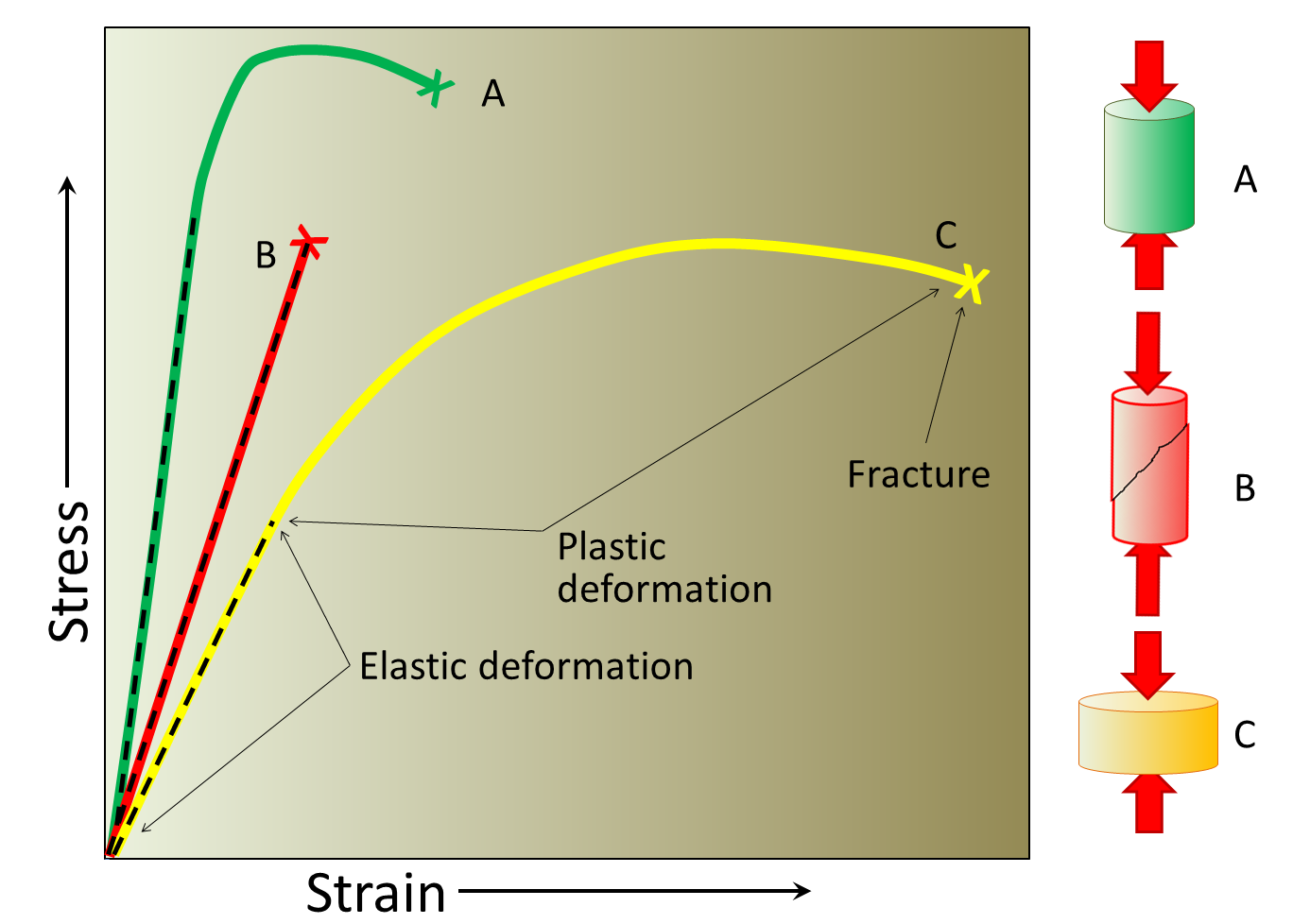
When rocks are stressed, the resulting strain can be elastic, ductile, or brittle. This change is generally called deformation. Elastic deformation is strain that is reversible after a stress is released. For example, when you stretch a rubber band, it elastically returns to its original shape after you release it. Ductile deformation occurs when enough stress is applied to a material that the changes in its shape are permanent, and the material is no longer able to revert to its original shape. For example, if you bend a metal bar too far, it can be permanently bent out of shape. The point at which elastic deformation is surpassed and strain becomes permanent is called the yield point. In the figure, yield point is where the line transitions from elastic deformation to ductile deformation (the end of the dashed line). Brittle deformation is another critical point of no return, when rock integrity fails and the rock fractures under increasing stress.
The type of deformation a rock undergoes depends on pore pressure, strain rate, rock strength, temperature, stress intensity, time, and confining pressure. Pore pressure is exerted on the rock by fluids in the open spaces or pores embedded within rock or sediment. Strain rate measures how quickly a material is deformed. For example, applying stress slowly makes it is easier to bend a piece of wood without breaking it. Rock strength measures how easily a rock deforms under stress. Shale has low strength and granite has high strength. Removing heat, or decreasing the temperature, makes materials more rigid and susceptible to brittle deformation. On the other hand, heating materials make them more ductile and less brittle. Heated glass can be bent and stretched.
| Factor | Strain response |
|---|---|
| Increase temperature | More ductile |
| Increase strain rate | More brittle |
| Increase rock strength | More brittle |
Table 9.2: Relationship between factors operating on rock and the resulting strains.

Take this quiz to check your comprehension of this section.
If you are using an offline version of this text, access the quiz for section 9.2 via the QR code.
9.3 Geological Maps
Geologic maps are two dimensional (2D) representations of geologic formations and structures at the Earth’s surface, including formations, faults, folds, inclined strata, and rock types. Formations are recognizable rock units. Geologists use geologic maps to represent where geologic formations, faults, folds, and inclined rock units are. Geologic formations are recognizable, mappable rock units. Each formation on the map is indicated by a color and a label. For examples of geologic maps, see the Utah Geological Survey (UGS) geologic map viewer.
Formation labels include symbols that follow a specific protocol. The first one or more letters are uppercase and represent the geologic time period of the formation. More than one uppercase letter indicates the formation is associated with multiple time periods. The following lowercase letters represent the formation name, abbreviated rock description, or both.
9.3.1 Cross Sections
Cross sections are subsurface interpretations made from surface and subsurface measurements. Maps display geology in the horizontal plane, while cross sections show subsurface geology in the vertical plane. For more information on cross sections, check out the AAPG wiki.
9.3.2 Strike and Dip
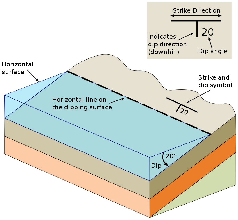
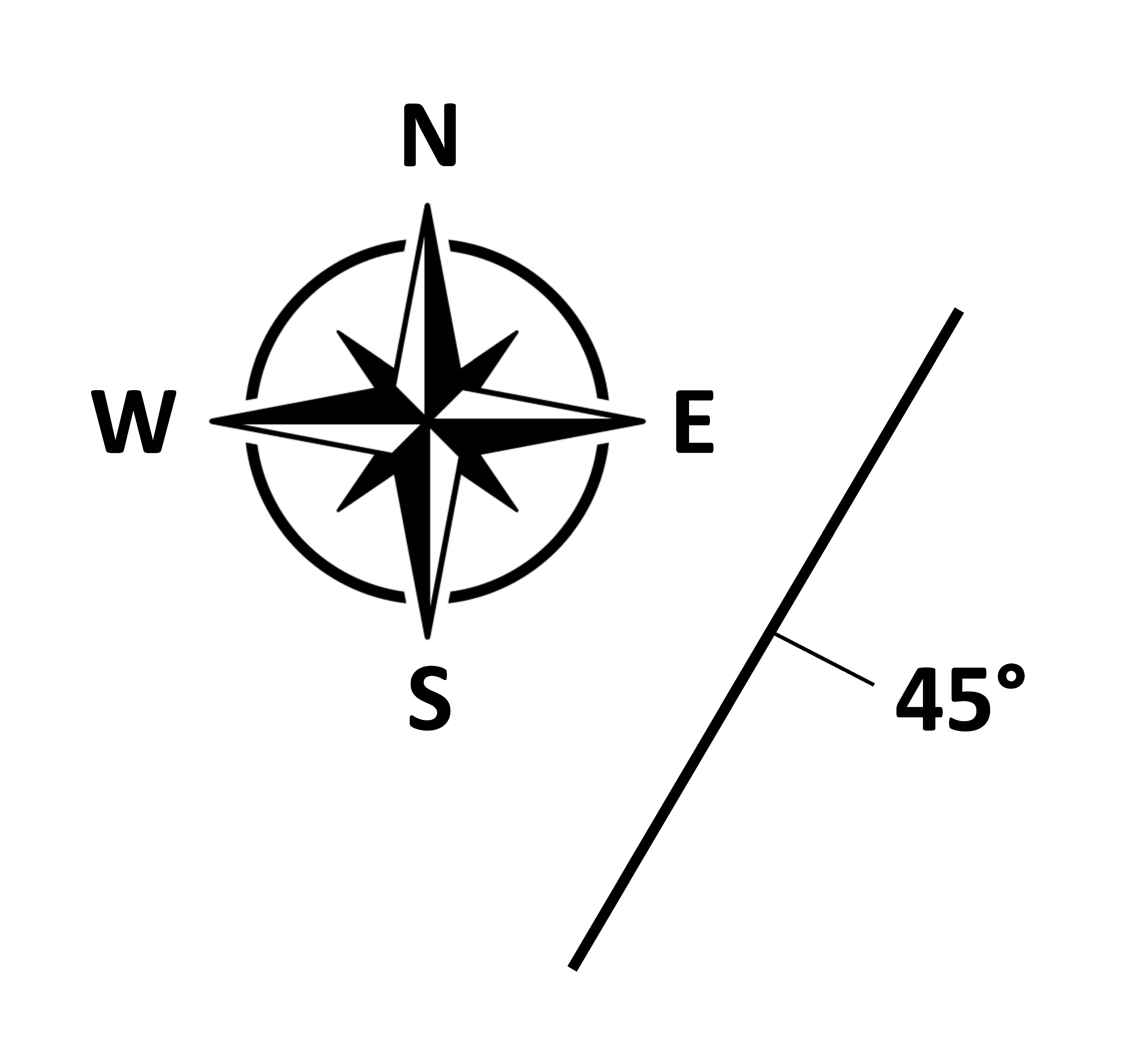
Geologists use a special symbol called strike and dip to represent inclined beds. Strike and dip map symbols look like the capital letter T, with a short trunk and extra-wide top line. The short trunk represents the dip and the top line represents the strike. Dip is the angle that a bed plunges into the Earth from the horizontal. A number next to the symbol represents dip angle. One way to visualize the strike is to think about a line made by standing water on the inclined layer. That line is horizontal and lies on a compass direction that has some angle with respect to true north or south (see figure 9.3). The strike angle is that angle measured by a special compass. E.g., N 30° E (read north 30 degrees east) means the horizontal line points northeast at an angle of 30° from true north. The strike and dip symbol is drawn on the map at the strike angle with respect to true north on the map. The dip of the inclined layer represents the angle down to the layer from horizontal, in the figure 45o SE (read dipping 45 degrees to the SE). The direction of dip would be the direction a ball would roll if set on the layer and released. A horizontal rock bed has a dip of 0° and a vertical bed has a dip of 90°. Strike and dip considered together are called rock attitude.
This video illustrates geologic structures and associated map symbols.

Video 9.1: Folds, dip, and strike.
If you are using an offline version of this text, access this YouTube video via the QR code.

Take this quiz to check your comprehension of this section.
If you are using an offline version of this text, access the quiz for section 9.3 via the QR code.
9.4 Folds
Geologic folds are layers of rock that are curved or bent by ductile deformation. Folds are most commonly formed by compressional forces at depth, where hotter temperatures and higher confining pressures allow ductile deformation to occur.
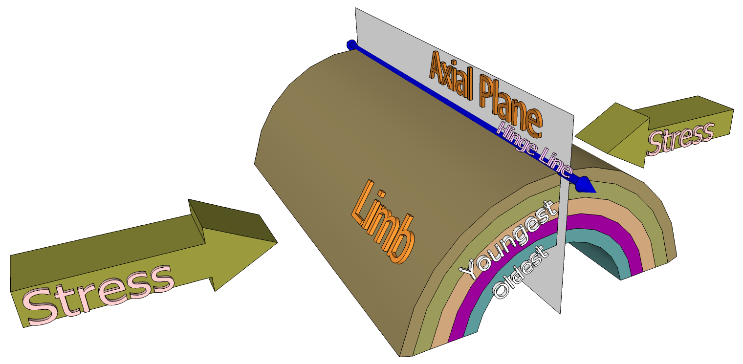
Folds are described by the orientation of their axes, axial planes, and limbs. The plane that splits the fold into two halves is known as the axial plane. The fold axis is the line along which the bending occurs and is where the axial plane intersects the folded strata. The hinge line follows the line of greatest bend in a fold. The two sides of the fold are the fold limbs.
Symmetrical folds have a vertical axial plane and limbs have equal but opposite dips. Asymmetrical folds have dipping, non-vertical axial planes, where the limbs dip at different angles. Overturned folds have steeply dipping axial planes and the limbs dip in the same direction but usually at different dip angles. Recumbent folds have horizontal or nearly horizontal axial planes. When the axis of the fold plunges into the ground, the fold is called a plunging fold. Folds are classified into five categories: anticline, syncline, monocline, dome, and basin.
9.4.1 Anticline
Anticlines are arch-like, or A-shaped, folds that are convex-upward in shape. They have downward curving limbs and beds that dip down and away from the central fold axis. In anticlines, the oldest rock strata are in the center of the fold, along the axis, and the younger beds are on the outside. Since geologic maps show the intersection of surface topography with underlying geologic structures, an anticline on a geologic map can be identified by both the attitude of the strata forming the fold and the older age of the rocks inside the fold. An antiform has the same shape as an anticline, but the relative ages of the beds in the fold cannot be determined. Oil geologists are interested in anticlines because they can form oil traps, where oil migrates up along the limbs of the fold and accumulates in the high point along the fold axis.
9.4.2 Syncline

3D Model 9.1: Synclinal fold.
If you are using an offline version of this text, access this interactive 3D model via the QR code, or visit https://sketchfab.com/3d-models/synclinal-fold-macigno-formation-3f0259ea2c6b4807a32fe3c950d13324.
Synclines are trough-like, or U shaped, folds that are concave-upward in shape. They have beds that dip down and in toward the central fold axis. In synclines, older rock is on the outside of the fold and the youngest rock is inside of the fold axis. A synform has the shape of a syncline but like an antiform, does not have distinguishable age zones.
9.4.3 Monocline
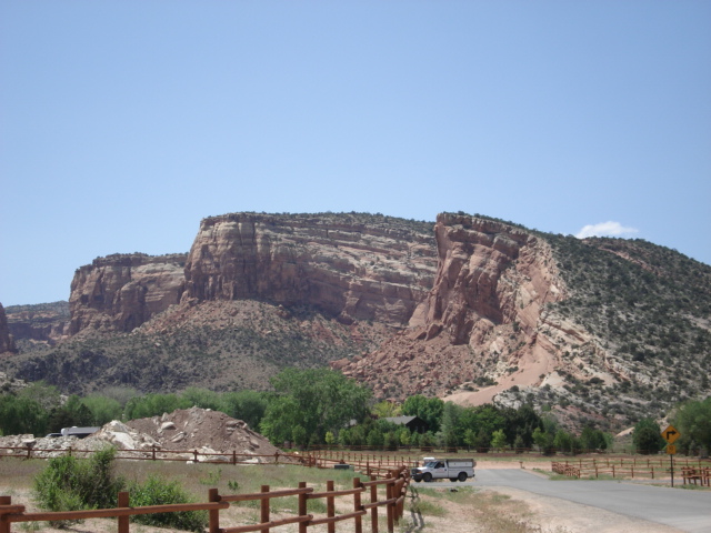
Monoclines are step-like folds, in which flat rocks are upwarped or downwarped, then continue flat. Monoclines are relatively common on the Colorado Plateau where they form “reefs,” which are ridges that act as topographic barriers and should not be confused with ocean reefs (see chapter 5). Capitol Reef is an example of a monocline in Utah. Monoclines can be caused by bending of shallower sedimentary strata as faults grow below them. These faults are commonly called “blind faults” because they end before reaching the surface and can be either normal or reverse faults.
9.4.4 Dome
A dome is a symmetrical to semi-symmetrical upwarping of rock beds. Domes have a shape like an inverted bowl, similar to an architectural dome on a building. Examples of domes in Utah include the San Rafael Swell, Harrisburg Junction Dome, and Henry Mountains. Domes are formed from compressional forces, underlying igneous intrusions (see chapter 4), by salt diapirs, or even impacts, like upheaval dome in Canyonlands National Park.
9.4.5 Basin
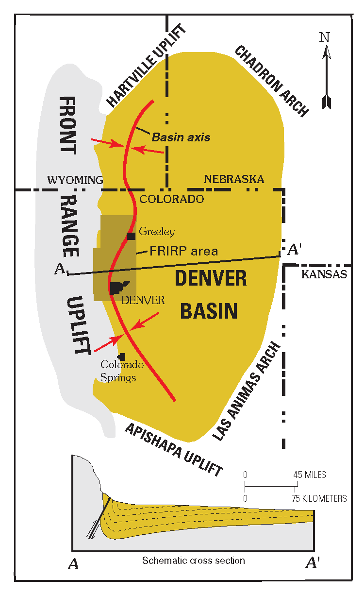
A basin is the inverse of a dome, a bowl-shaped depression in a rock bed. The Uinta Basin in Utah is an example of a basin. Some structural basins are also sedimentary basins that collect large quantities of sediment over time. Sedimentary basins can form as a result of folding but are much more commonly produced in mountain building, forming between mountain blocks or via faulting. Regardless of the cause, as the basin sinks or subsides, it can accumulate more sediment because the weight of the sediment causes more subsidence in a positive-feedback loop. There are active sedimentary basins all over the world. An example of a rapidly subsiding basin in Utah is the Oquirrh Basin, dated to the Pennsylvanian-Permian age, which has accumulated over 9,144 m (30,000 ft) of fossiliferous sandstones, shales, and limestones. These strata can be seen in the Wasatch Mountains along the east side of Utah Valley, especially on Mt. Timpanogos and in Provo Canyon.

Take this quiz to check your comprehension of this section.
If you are using an offline version of this text, access the quiz for section 9.4 via the QR code.
9.5 Faults
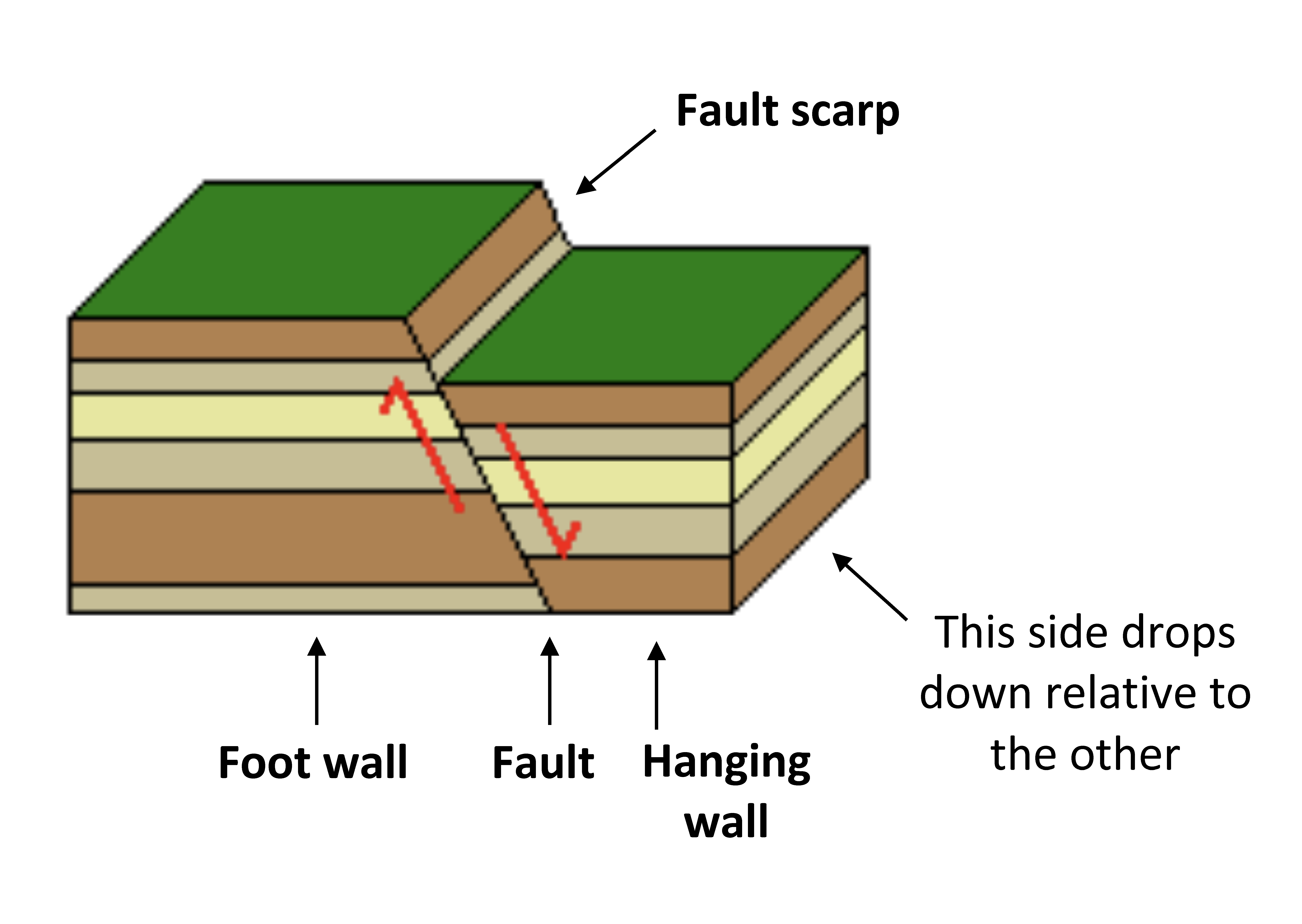
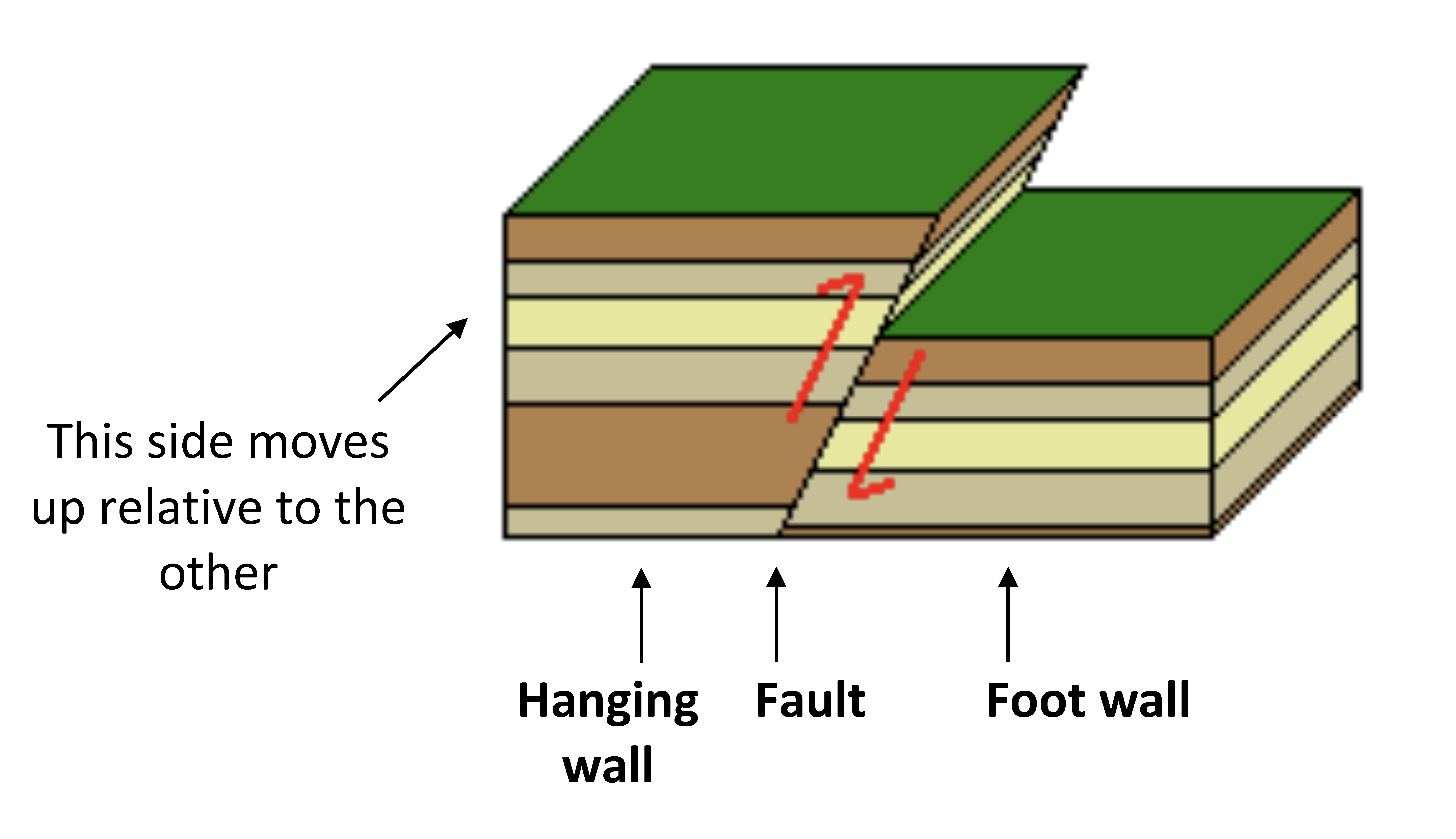
Faults are the places in the crust where brittle deformation occurs as two blocks of rocks move relative to one another. Normal and reverse faults display vertical, also known as dip-slip, motion. Dip-slip motion consists of relative up-and-down movement along a dipping fault between two blocks, the hanging wall and footwall. In a dip-slip system, the footwall is below the fault plane and the hanging wall is above the fault plane. A good way to remember this is to imagine a mine tunnel running along a fault; the hanging wall would be where a miner would hang a lantern and the footwall would be at the miner’s feet.
Faulting as a term refers to rupture of rocks. Such ruptures occur at plate boundaries but can also occur in plate interiors as well. Faults slip along the fault plane. The fault scarp is the offset of the surface produced where the fault breaks through the surface. Slickensides are polished, often grooved surfaces along the fault plane created by friction during the movement.
A joint or fracture is a plane of brittle deformation in rock created by movement that is not offset or sheared. Joints can result from many processes, such as cooling, depressurizing, or folding. Joint systems may be regional affecting many square miles.
9.5.1 Normal Faults
Normal faults move by a vertical motion where the hanging-wall moves downward relative to the footwall along the dip of the fault. Normal faults are created by tensional forces in the crust. Normal faults and tensional forces commonly occur at divergent plate boundaries, where the crust is being stretched by tensional stresses (see chapter 2). Examples of normal faults in Utah are the Wasatch Fault, the Hurricane Fault, and other faults bounding the valleys in the Basin and Range province.
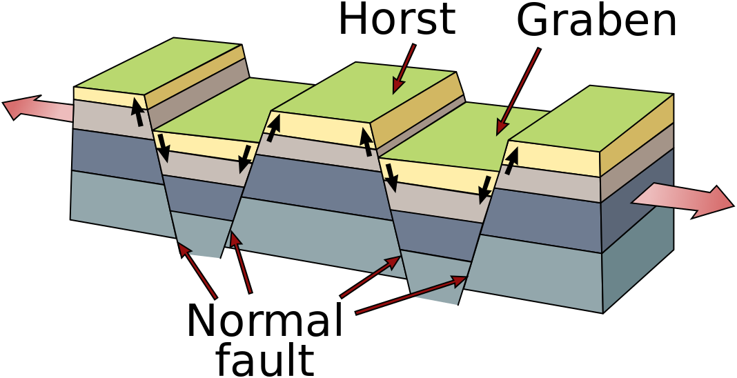
Grabens, horsts, and half-grabens are blocks of crust or rock bounded by normal faults (see chapter 2). Grabens drop down relative to adjacent blocks and create valleys. Horsts rise up relative to adjacent down-dropped blocks and become areas of higher topography. Where occurring together, horsts and grabens create a symmetrical pattern of valleys surrounded by normal faults on both sides and mountains. Half-grabens are a one-sided version of a horst and graben, where blocks are tilted by a normal fault on one side, creating an asymmetrical valley-mountain arrangement. The mountain-valleys of the Basin and Range Province of Western Utah and Nevada consist of a series of full and half-grabens from the Salt Lake Valley to the Sierra Nevada Mountains.
Normal faults do not continue clear into the mantle. In the Basin and Range Province, the dip of a normal fault tends to decrease with depth, i.e., the fault angle becomes shallower and more horizontal as it goes deeper. Such decreasing dips happen when large amounts of extension occur along very low-angle normal faults, known as detachment faults. The normal faults of the Basin and Range, produced by tension in the crust, appear to become detachment faults at greater depths.
9.5.2 Reverse Faults
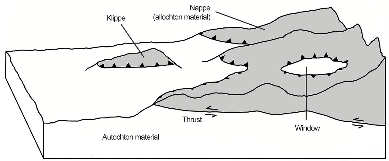
In reverse faults, compressional forces cause the hanging wall to move up relative to the footwall. A thrust fault is a reverse fault where the fault plane has a low dip angle of less than 45°. Thrust faults carry older rocks on top of younger rocks and can even cause repetition of rock units in the stratigraphic record.
Convergent plate boundaries with subduction zones create a special type of “reverse” fault called a megathrust fault where denser oceanic crust drives down beneath less dense overlying crust. Megathrust faults cause the largest magnitude earthquakes yet measured and commonly cause massive destruction and tsunamis.
9.5.3 Strike–Slip Faults
Strike-slip faults have side-to-side motion. Strike-slip faults are most commonly associated with transform plate boundaries and are prevalent in transform fracture zones along mid-ocean ridges. In pure strike-slip motion, fault blocks on either side of the fault do not move up or down relative to each other, rather move laterally, side to side. The direction of strike-slip movement is determined by an observer standing on a block on one side of the fault. If the block on the opposing side of the fault moves left relative to the observer’s block, this is called sinistral motion. If the opposing block moves right, it is dextral motion.

Video 9.2: Video showing motion in a strike-slip fault.
If you are using an offline version of this text, access this YouTube video via the QR code.
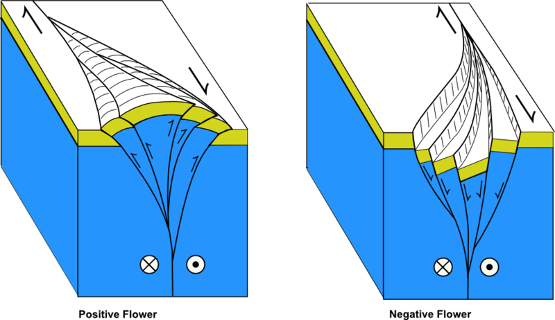
Bends along strike-slip faults create areas of compression or tension between the sliding blocks (see chapter 2). Tensional stresses create transtensional features with normal faults and basins, such as the Salton Sea in California. Compressional stresses create transpressional features with reverse faults and cause small-scale mountain building, such as the San Gabriel Mountains in California. The faults that splay off transpression or transtension features are known as flower structures.
An example of a dextral, right-lateral strike-slip fault is the San Andreas Fault, which denotes a transform boundary between the North American and Pacific plates. An example of a sinistral, left-lateral strike-slip fault is the Dead Sea fault in Jordan and Israel.

Video 9.3: Video showing how faults are classified.
If you are using an offline version of this text, access this YouTube video via the QR code.

Take this quiz to check your comprehension of this section.
If you are using an offline version of this text, access the quiz for section 9.5 via the QR code.
9.6 Earthquake Essentials
Earthquakes are felt at the surface of the Earth when energy is released by blocks of rock sliding past each other, i.e. faulting has occurred. Seismic energy thus released travels through the Earth in the form of seismic waves. Most earthquakes occur along active plate boundaries. Intraplate earthquakes (not along plate boundaries) occur and are still poorly understood. The USGS Earthquakes Hazards Program has a real time map showing the most recent earthquakes.
9.6.1 How Earthquakes Happen
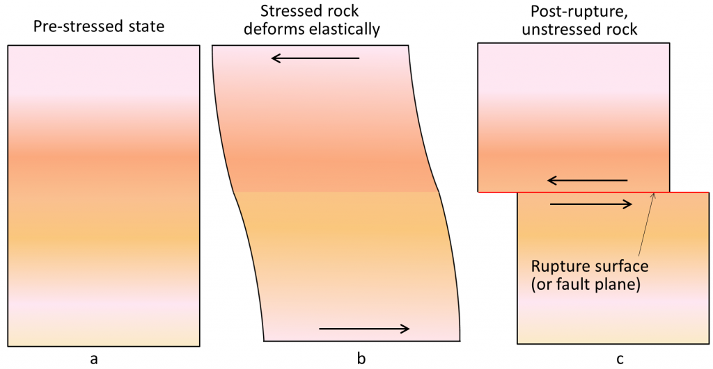
The release of seismic energy is explained by the elastic rebound theory. When rock is strained to the point that it undergoes brittle deformation, The place where the initial offsetting rupture takes place between the fault blocks is called the focus. This offset propagates along the fault, which is known as the fault plane.
The fault blocks of persistent faults like the Wasatch Fault (Utah), that show recurring movements, are locked together by friction. Over hundreds to thousands of years, stress builds up along the fault until it overcomes frictional resistance, rupturing the rock and initiating fault movement. The deformed unbroken rocks snap back toward their original shape in a process called elastic rebound. Think of bending a stick until it breaks; stored energy is released, and the broken pieces return to near their original orientation.
Bending, the ductile deformation of the rocks near a fault, reflects a build-up of stress. In earthquake-prone areas like California, strain gauges are used to measure this bending and help seismologists, scientists who study earthquakes, understand more about predicting them. In locations where the fault is not locked, seismic stress causes continuous, gradual displacement between the fault blocks called fault creep. Fault creep occurs along some parts of the San Andreas Fault (California).
After an initial earthquake, continuous application of stress in the crust causes elastic energy to begin to build again during a period of inactivity along the fault. The accumulating elastic strain may be periodically released to produce small earthquakes on or near the main fault called foreshocks. Foreshocks can occur hours or days before a large earthquake, or may not occur at all. The main release of energy during the major earthquake is known as the mainshock. Aftershocks may follow the mainshock to adjust new strain produced during the fault movement and generally decrease over time.
9.6.2 Focus and Epicenter
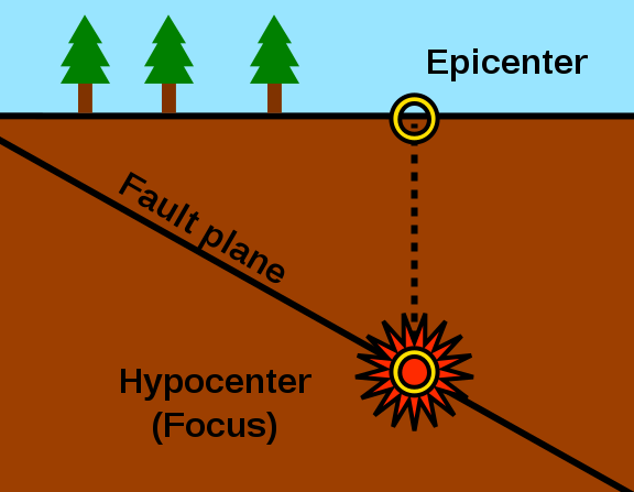
The earthquake focus, also called hypocenter, is the initial point of rupture and displacement of the rock moves from the hypocenter along the fault surface. The earthquake focus or hypocenter is the point along the fault plane from which initial seismic waves spread outward and is always at some depth below the ground surface. From the focus, rock displacement propagates up, down, and laterally along the fault plane. This displacement produces shock waves called seismic waves. The larger the displacement between the opposing fault blocks and the further the displacement propagates along the fault surface, the more seismic energy is released and the greater the amount and time of shaking is produced. The epicenter is the location on the Earth’s surface vertically above the focus. This is the location that most news reports give because it is the center of the area where people are affected.
9.6.3 Seismic Waves
To understand earthquakes and how earthquake energy moves through the Earth, consider the basic properties of waves. Waves describe how energy moves through a medium, such as rock or unconsolidated sediments in the case of earthquakes. Wave amplitude indicates the magnitude or height of earthquake motion. Wavelength is the distance between two successive peaks of a wave. Wave frequency is the number of repetitions of the motion over a period of time, cycles per time unit. Period, which is the amount of time for a wave to travel one wavelength, is the inverse of frequency. When multiple waves combine, they can interfere with each other (see figure 9.19). When waves combine in sync, they produce constructive interference, where the influence of one wave adds to and magnifies the other. If waves are out of sync, they produce destructive interference, which diminishes the amplitudes of both waves. If two combined waves have the same amplitude and frequency but are one-half wavelength out of sync, the resulting destructive interference can eliminate each wave. These processes of wave amplitude, frequency, period, and constructive and destructive interference determine the magnitude and intensity of earthquakes.
Seismic waves are the physical expression of energy released by the elastic rebound of rock within displaced fault blocks and are felt as an earthquake. Seismic waves occur as body waves and surface waves. Body waves pass underground through the Earth’s interior body and are the first seismic waves to propagate out from the focus. Body waves include primary (P) waves and secondary (S) waves. P waves are the fastest body waves and move through rock via compression, very much like sound waves move through air. Rock particles move forward and back during passage of the P waves, enabling them to travel through solids, liquids, plasma, and gases. S waves travel slower, following P waves, and propagate as shear waves that move rock particles from side to side. Because they are restricted to lateral movement, S waves can only travel through solids but not liquids, plasma, or gases.
During an earthquake, body waves pass through the Earth and into the mantle as a sub-spherical wave front. Considering a point on a wave front, the path followed by a specific point on the spreading wave front is called a seismic ray and a seismic ray reaches a specific seismograph located at one of thousands of seismic monitoring stations scattered over the Earth. Density increases with depth in the Earth, and since seismic velocity increases with density, a process called refraction causes earthquake rays to curve away from the vertical and bend back toward the surface, passing through different bodies of rock along the way.
Surface waves are produced when body waves from the focus strike the Earth’s surface. Surface waves travel along the Earth’s surface, radiating outward from the epicenter. Surface waves take the form of rolling waves called Raleigh Waves and side to side waves called Love Waves (watch videos for wave propagation animations). Surface waves are produced primarily as the more energetic S waves strike the surface from below with some surface wave energy contributed by P waves (videos courtesy blog.Wolfram.com). Surface waves travel more slowly than body waves and because of their complex horizontal and vertical movement, surface waves are responsible for most of the damage caused by an earthquake. Love waves produce predominantly horizontal ground shaking and, ironically from their name, are the most destructive. Rayleigh waves produce an elliptical motion with longitudinal dilation and compression, like ocean waves. However, Raleigh waves cause rock particles to move in a direction opposite to that of water particles in ocean waves.
The Earth has been described as ringing like a bell after an earthquake with earthquake energy reverberating inside it. Like other waves, seismic waves refract (bend) and bounce (reflect) when passing through rocks of differing densities. S waves, which cannot move through liquid, are blocked by the Earth’s liquid outer core, creating an S wave shadow zone on the side of the planet opposite to the earthquake focus. P waves, on the other hand, pass through the core, but are refracted into the core by the difference of density at the core–mantle boundary. This has the effect of creating a cone shaped P wave shadow zone on parts of the other side of the Earth from the focus.

Video 9.4: Body and surface waves of 2011 Tohoku earthquake.
If you are using an offline version of this text, access this video via the QR code.
9.6.4 Induced Seismicity
Earthquakes known as induced seismicity occur near natural gas extraction sites because of human activity. Injection of waste fluids in the ground, commonly a byproduct of an extraction process for natural gas known as fracking, can increase the outward pressure that liquid in the pores of a rock exerts, known as pore pressure. The increase in pore pressure decreases the frictional forces that keep rocks from sliding past each other, essentially lubricating fault planes. This effect is causing earthquakes to occur near injection sites, in a human induced activity known as induced seismicity. The significant increase in drilling activity in the central United States has spurred the requirement for the disposal of significant amounts of waste drilling fluid, resulting in a measurable change in the cumulative number of earthquakes experienced in the region.

Take this quiz to check your comprehension of this section.
If you are using an offline version of this text, access the quiz for section 9.6 via the QR code.
9.7 Measuring Earthquakes
9.7.1 Seismographs

Video 9.5: Animation of a horizontal seismograph.
If you are using an offline version of this text, access this YouTube video via the QR code.
People feel approximately 1 million earthquakes a year, usually when they are close to the source and the earthquake registers at least moment magnitude 2.5. Major earthquakes of moment magnitude 7.0 and higher are extremely rare. The U. S. Geological Survey (USGS) Earthquakes Hazards Program real-time map shows the location and magnitude of recent earthquakes around the world.
To accurately study seismic waves, geologists use seismographs that can measure even the slightest ground vibrations. Early 20th-century seismograms use a weighted pen (pendulum) suspended by a long spring above a recording device fixed solidly to the ground. The recording device is a rotating drum mounted with a continuous strip of paper. During an earthquake, the suspended pen stays motionless and records ground movement on the paper strip. The resulting graph a seismogram. Digital versions use magnets, wire coils, electrical sensors, and digital signals instead of mechanical pens, springs, drums, and paper. A seismograph array is multiple seismographs configured to measure vibrations in three directions: north-south (x axis), east-west (y axis), and up-down (z axis).

Video 9.6: Animation of a vertical seismograph.
If you are using an offline version of this text, access this YouTube video via the QR code.
To pinpoint the location of an earthquake epicenter, seismologists use the differences in arrival times of the P, S, and surface waves. After an earthquake, P waves will appear first on a seismogram, followed by S waves, and finally surface waves, which have the largest amplitude. It is important to note that surface waves lose energy quickly, so they are not measurable at great distances from the epicenter. These time differences determine the distance but not the direction of the epicenter. By using wave arrival times recorded on seismographs at multiple stations, seismologists can apply triangulation to pin point the location of the epicenter of an earthquake. At least three seismograph stations are needed for triangulation. The distance from each station to the epicenter is plotted as the radius of a circle. The epicenter is demarked where the circles intersect. This method also works in 3D, using multi-axis seismographs and sphere radii to calculate the underground depth of the focus.

Video 9.7: This video shows the method of triangulation to locate the epicenter of an earthquake.
If you are using an offline version of this text, access this YouTube video via the QR code.
9.7.2 Seismograph Network
The International Registry of Seismograph Stations lists more than 20,000 seismographs on the planet. By comparing data from multiple seismographs, scientists can map the properties of the inside of the Earth, detect detonations of large explosive devices, and predict tsunamis. The Global Seismic Network, a worldwide set of linked seismographs that electronically distribute real-time data, includes more than 150 stations that meet specific design and precision standards. The USArray is a network of hundreds of permanent and transportable seismographs in the United States that are used to map the subsurface activity of earthquakes (see video).
Along with monitoring for earthquakes and related hazards, the Global Seismograph Network helps detect nuclear weapons testing, which is monitored by the Comprehensive Nuclear Test Ban Treaty Organization. Most recently, seismographs have been used to determine nuclear weapons testing by North Korea.

Video 9.8: Nepal earthquake (M7.9) ground motion visualization.
If you are using an offline version of this text, access this YouTube video via the QR code.
9.7.3 Seismic Tomography
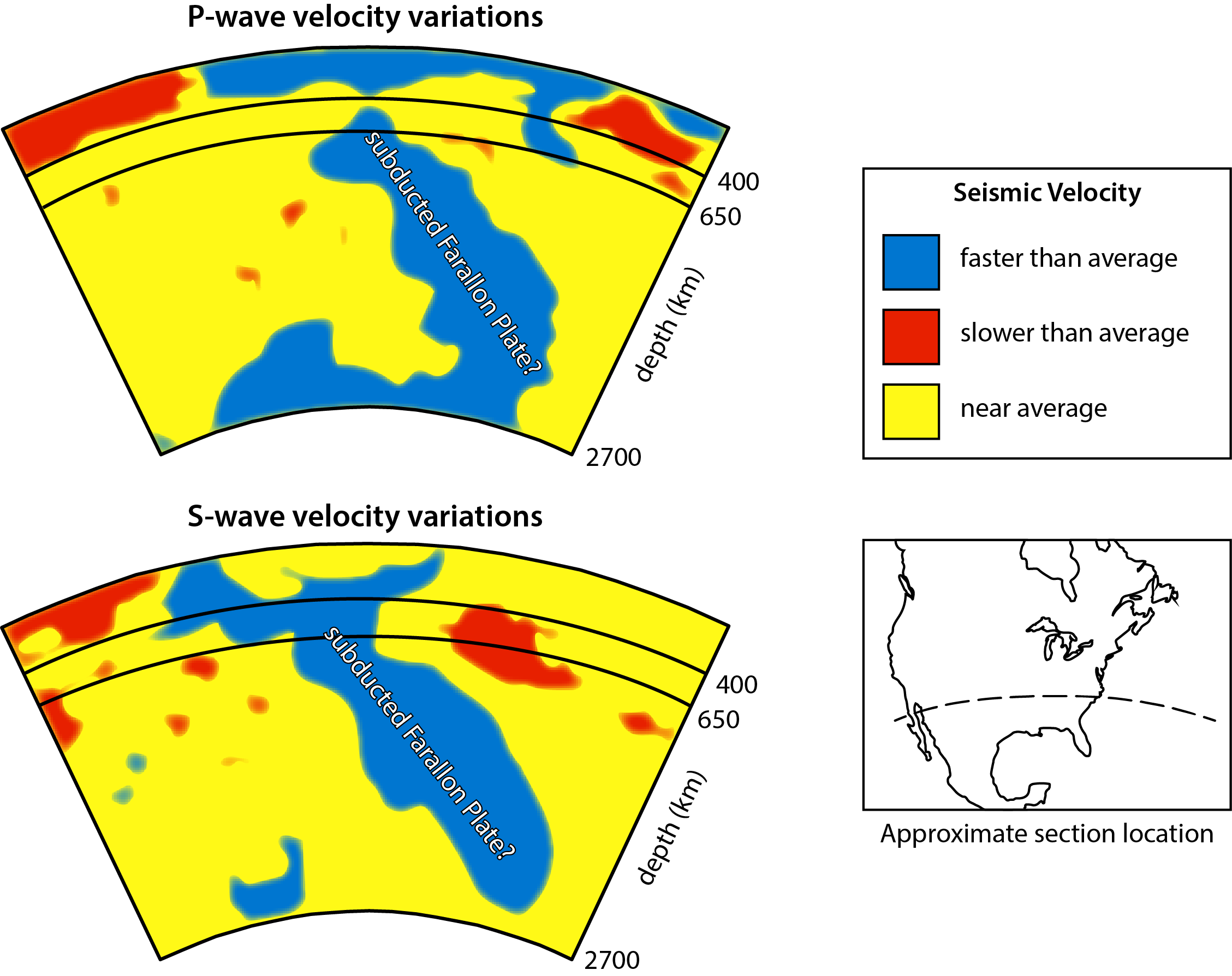
Very much like a CT (Computed Tomography) scan uses X-rays at different angles to image the inside of a body, seismic tomography uses seismic rays from thousands of earthquakes that occur each year, passing at all angles through masses of rock, to generate images of internal Earth structures.
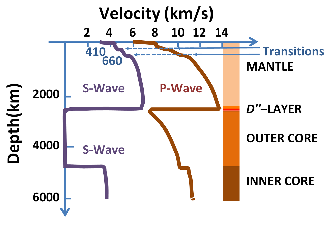
Using the assumption that the earth consists of homogenous layers, geologists developed a model of expected properties of earth materials at every depth within the earth called the PREM (Preliminary Reference Earth Model). These properties include seismic wave transmission velocity, which is dependent on rock density and elasticity. In the mantle, temperature differences affect rock density. Cooler rocks have a higher density and therefore transmit seismic waves faster. Warmer rocks have a lower density and transmit earthquake waves slower. When the arrival times of seismic rays at individual seismic stations are compared to arrival times predicted by PREM, differences are called seismic anomalies and can be measured for bodies of rock within the earth from seismic rays passing through them at stations of the seismic network. Because seismic rays travel at all angles from lots of earthquakes and arrive at lots of stations of the seismic network, like CT scans of the body, variations in the properties of the rock bodies allow 3D images to be constructed of the rock bodies through which the rays passed. Seismologists are thus able to construct 3D images of the interior of the Earth..
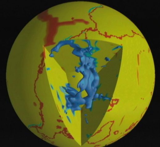
For example, seismologists have mapped the Farallon Plate, a tectonic plate that subducted beneath North America during the last several million years, and the Yellowstone magma chamber, which is a product of the Yellowstone hot spot under the North American continent. Peculiarities of the Farallon Plate subduction are thought to be responsible for many features of western North America including the Rocky Mountains (see chapter 8).
9.7.4 Earthquake Magnitude and Intensity
Richter Scale
Magnitude is the measure of the energy released by an earthquake. The Richter scale (ML), the first and most well-known magnitude scale, was developed by Charles F. Richter (1900-1985) at the California Institute of Technology. This was the magnitude scale used historically by early seismologists. Used by early seismologists, Richter magnitude (ML) is determined from the maximum amplitude of the pen tracing on the seismogram recording. Adjustments for epicenter distance from the seismograph are made using the arrival-time differences of S and P waves.
The Richter Scale is logarithmic, based on powers of 10. This means an increase of one Richter unit represents a 10-fold increase in seismic-wave amplitude or in other words, a magnitude 6 earthquake shakes the ground 10 times more than a magnitude 5. However, the actual energy released for each magnitude unit is 32 times greater, which means a magnitude 6 earthquake releases 32 times more energy than a magnitude 5.
The Richter Scale was developed for earthquakes in Southern California, using local seismographs. It has limited applications for larger distances and very large earthquakes. Therefore, most agencies no longer use the Richter Scale. Moment magnitude (MW), which is measured using seismic arrays and generates values comparable to the Richter Scale, is more accurate for measuring earthquakes across the Earth, including large earthquakes, although they require more time to calculate. News media often report Richter magnitudes right after an earthquake occurs even though scientific calculations now use moment magnitudes.
Moment Magnitude Scale
The moment magnitude scale depicts the absolute size of earthquakes, comparing information from multiple locations and using a measurement of actual energy released calculated from cross-sectional area of rupture, amount of slippage, and the rigidity of the rocks. Because each earthquake occurs in a unique geologic setting and the rupture area is often hard to measure, estimates of moment magnitude can take days or even months to calculate.
Like the Richter Scale, the moment magnitude scale is logarithmic. Magnitude values of the two scales are approximately equal, except for very large earthquakes. Both scales are used for reporting earthquake magnitude. The Richter Scale provides a quick magnitude estimate immediately following the quake and thus, is usually reported in news accounts. Moment magnitude calculations take much longer but are more accurate and thus, more useful for scientific analysis.

Video 9.9: Moment magnitude explained.
If you are using an offline version of this text, access this YouTube video via the QR code.
Modified Mercalli Intensity Scale
The Modified Mercalli Intensity Scale (MMI) is a qualitative rating of ground-shaking intensity based on observable structural damage and people’s perceptions. This scale uses a I (Roman numeral one) rating for the lowest intensity and X (ten) for the highest (see table) and can vary depending on epicenter location and population density, such as urban versus rural settings. Historically, scientists used the MMI Scale to categorize earthquakes before they developed quantitative measurements of magnitude. Intensity maps show locations of the most severe damage, based on residential questionnaires, local news articles, and on-site assessment reports.
| Intensity | Shaking | Description/damage |
|---|---|---|
| I | Not felt | Not felt except by a very few under especially favorable conditions. |
| II | Weak | Felt only by a few persons at rest, especially on upper floors of buildings. |
| III | Weak | Felt quite noticeably by persons indoors, especially on upper floors of buildings. Many people do not recognize it as an earthquake. Standing motor cars may rock slightly. Vibrations similar to the passing of a truck. Duration estimated. |
| IV | Light | Felt indoors by many, outdoors by few during the day. At night, some awakened. Dishes, windows, doors disturbed; walls make cracking sound. Sensation like heavy truck striking building. Standing motor cars rocked noticeably. |
| V | Moderate | Felt by nearly everyone; many awakened. Some dishes, windows broken. Unstable objects overturned. Pendulum clocks may stop. |
| VI | Strong | Felt by all, many frightened. Some heavy furniture moved; a few instances of fallen plaster. Damage slight. |
| VII | Very strong | Damage negligible in buildings of good design and construction; slight to moderate in well-built ordinary structures; considerable damage in poorly built or badly designed structures; some chimneys broken. |
| VIII | Severe | Damage slight in specially designed structures; considerable damage in ordinary substantial buildings with partial collapse. Damage great in poorly built structures. Fall of chimneys, factory stacks, columns, monuments, walls. Heavy furniture overturned. |
| IX | Violent | Damage considerable in specially designed structures; well-designed frame structures thrown out of plumb. Damage great in substantial buildings, with partial collapse. Buildings shifted off foundations. |
| X | Extreme | Some well-built wooden structures destroyed; most masonry and frame structures destroyed with foundations. Rails bent. |
Table 9.3: Abridged Mercalli Scale from USGS General Interest Publication 1989-288-913.
Shake Maps
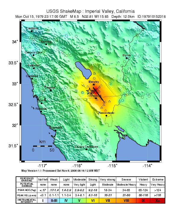
Shake maps, written ShakeMaps by the USGS, use high-quality, computer-interpolated data from seismograph networks to show areas of intense shaking. Shake maps are useful in the crucial minutes after an earthquake, as they show emergency personnel where the greatest damage likely occurred and help them locate possibly damaged gas lines and other utility facilities.

Take this quiz to check your comprehension of this section.
If you are using an offline version of this text, access the quiz for section 9.7 via the QR code.
9.8 Earthquake Risk
9.8.1 Factors That Determine Shaking
Earthquake magnitude is an absolute value that measures pure energy release. Intensity however, i.e. how much the ground shakes, is a determined by several factors.
Earthquake magnitude—In general, the larger the magnitude, the stronger the shaking and the longer the shaking will last.
This table is taken from from the USGS and shows scales of magnitude and Mercalli Intensity, and descriptions of shaking and resulting damage.
| Magnitude | Modified Mercalli Intensity | Shaking/damage description |
|---|---|---|
| 1.0-3.0 | I | Only felt by a very few. |
| 3.0-3.9 | II-III | Noticeable indoors, especially on upper floors. |
| 4.0-4.9 | IV-V | Most to all feel it. Dishes, doors, cars shake and possibly break. |
| 5.0-5.9 | VI-VII | Everyone feels it. Some items knocked over or broken. Building damage possible. |
| 6.0-6.9 | VII-IX | Frightening amounts of shaking. Significant damage especially with poorly constructed buildings. |
| ≥ 7.0 | ≥ VIII | Significant destruction of buildings. Potential for objects to be thrown in air from shaking. |
Table 9.4: Mercalli Intensity as it relates to magnitude.
Location and direction—Shaking is more severe closer to the epicenter. The severity of shaking is influenced by the location of the observer relative to epicenter, direction of rupture propagation, and path of greatest rupture.
Local geologic conditions—Seismic waves are affected by the nature of the ground materials through which they pass. Different materials respond differently to an earthquake. Think of shaking a block of Jello versus a meatloaf, one will jiggle much more when hit by waves of the same amplitude. The ground’s response to shaking depends on the degree of substrate consolidation. Solid sedimentary, igneous, or metamorphic bedrock shakes less than unconsolidated sediments.

Video 9.10: This video shows how different substrates behave in response to different seismic waves and their potential for destruction.
If you are using an offline version of this text, access this YouTube video via the QR code.
Seismic waves move fastest through consolidated bedrock, slower through unconsolidated sediments, and slowest through unconsolidated sediments with a high water content. Seismic energy is transmitted by wave velocity and amplitude. When seismic waves slow down, energy is transferred to the amplitude, increasing the motion of surface waves, which in turn amplifies ground shaking.
Focus depth—Deeper earthquakes cause less surface shaking because much of their energy, transmitted as body waves, is lost before reaching the surface. Recall that surface waves are generated by P and S waves impacting the Earth’s surface.
9.8.2 Factors that Determine Destruction
Just as certain conditions will impact intensity of ground-shaking, several factors affect how much destruction is caused.
Building materials—The flexibility of a building material determines its resistance to earthquake damage. Unreinforced masonry (URM) is the material most devastated by ground shaking. Wood framing fastened with nails bends and flexes during seismic wave passage and is more likely to survive intact. Steel also has the ability to deform elastically before brittle failure. The Fix the Bricks campaign in Salt Lake City, Utah has good information on URMs and earthquake safety.
Intensity and duration—Greater shaking and duration of shaking causes more destruction than lower and shorter shaking.
Resonance—Resonance occurs when seismic wave frequency matches a building’s natural shaking frequency and increases the shaking happened in the 1985 Mexico City Earthquake, where buildings of heights between 6 and 15 stories were especially vulnerable to earthquake damage. Skyscrapers designed with earthquake resilience have dampers and base isolation features to reduce resonance.
Resonance is influenced by the properties of the building materials. Changes in the structural integrity of a building can alter resonance. Conversely, changes in measured resonance can indicate a potentially altered structural integrity.
These two videos discuss why buildings fall during earthquakes and a modern procedure to reduce potential earthquake destruction for larger buildings.

Video 9.11: Why do buildings fall in earthquakes?
If you are using an offline version of this text, access this YouTube video via the QR code.

Video 9.12: Base isolators.
If you are using an offline version of this text, access this YouTube video via the QR code.
9.8.3 Earthquake Recurrence
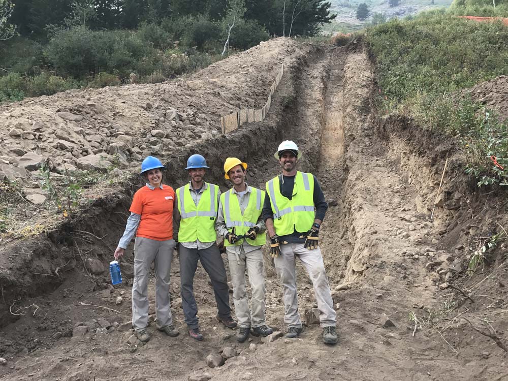
A long hiatus in activity on along a fault segment with a history of recurring earthquakes is known as a seismic gap. The lack of activity may indicate the fault segment is locked, which may produce a buildup of strain and higher probability of an earthquake recurring. Geologists dig earthquake trenches across faults to estimate the frequency of past earthquake occurrences. Trenches are effective for faults with relatively long recurrence intervals, roughly 100s to 10,000s of years between significant earthquakes. Trenches are less useful in areas with more frequent earthquakes because they usually have more recorded data.
9.8.4 Earthquake Distribution
This video shows the distribution of significant earthquakes on the Earth during the years 2010 through 2012. Like volcanoes, earthquakes tend to aggregate around active boundaries of tectonic plates. The exception is intraplate earthquakes, which are comparatively rare.
https://youtube.com/watch?v=Wc6vtj4yYcY

Video 9.13: 2010-2012 Earthquake visualization map.
If you are using an offline version of this text, access this YouTube video via the QR code.
Subduction zones—Subduction zones, found at convergent plate boundaries, are where the largest and deepest earthquakes, called megathrust earthquakes, occur. Examples of subduction-zone earthquake areas include the Sumatran Islands, Aleutian Islands, west coast of South America, and Cascadia Subduction Zone off the coast of Washington and Oregon. See chapter 2 for more information about subduction zones.
Collision zones—Collisions between converging continental plates create broad earthquake zones that may generate deep, large earthquakes from the remnants of past subduction events or other deep-crustal processes. The Himalayan Mountains (northern border of the Indian subcontinent) and Alps (southern Europe and Asia) are active regions of collision-zone earthquakes. See chapter 2 for more information about collision zones.
Transform boundaries—Strike-slip faults created at transform boundaries produce moderate-to-large earthquakes, usually having a maximum moment magnitude of about 8. The San Andreas Fault (California) is an example of a transform-boundary earthquake zone. Haiti’s Enriquillo-Plantain Garden fault system, which caused the 2010 earthquake near Port-au-Prince (see below), and Septentrional Fault, which destroyed Cap-Haïtien in 1842 and shook Cuba in 2020, are also transform faults. Other examples are the Alpine Fault (New Zealand) and Anatolian Faults (Turkey). See chapter 2 for more information about transform boundaries.
Divergent boundaries—Continental rifts and mid-ocean ridges found at divergent boundaries generally produce moderate earthquakes. Examples of active earthquake zones include the East African Rift System (southwestern Asia through eastern Africa), Iceland, and Basin and Range province (Nevada, Utah, California, Arizona, and northwestern Mexico). See chapter 2 for more information about divergent boundaries.
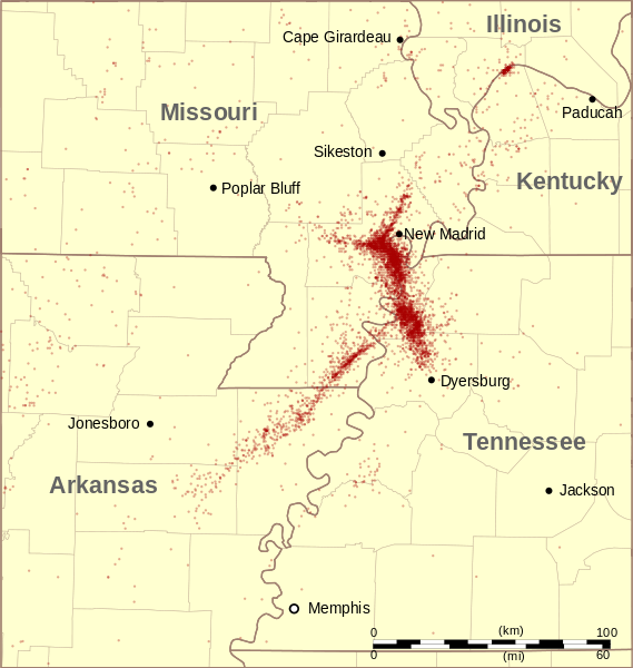
Intraplate earthquakes—Intraplate earthquakes are not found near tectonic plate boundaries, but generally occur in areas of weakened crust or concentrated tectonic stress. The New Madrid seismic zone, which covers Missouri, Illinois, Tennessee, Arkansas, and Indiana, is thought to represent the failed Reelfoot rift. The failed rift zone weakened the crust, making it more responsive to tectonic plate movement and interaction. Geologists theorize the infrequently occurring earthquakes are produced by low strain rates
9.8.5 Secondary Hazards Caused by Earthquakes
Most earthquake damage is caused by ground shaking and fault block displacement. In addition, there are secondary hazards that endanger structures and people, in some cases after the shaking stops.
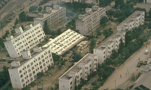
Buildings toppled from liquefaction during a 7.5 magnitude earthquake in Japan.
Liquefaction—Liquefaction occurs when water-saturated, unconsolidated sediments, usually silt or sand, become fluid-like from shaking. The shaking breaks the cohesion between grains of sediment, creating a slurry of particles suspended in water. Buildings settle or tilt in the liquified sediment, which looks very much like quicksand in the movies. Liquefaction also creates sand volcanoes, cone-shaped features created when liquefied sand is squirted through an overlying and usually finer-grained layer.

Video 9.14: This video demonstrates how liquefaction takes place.
If you are using an offline version of this text, access this YouTube video via the QR code.
This video shows liquefaction occurring during the 2011 earthquake in Japan.

Video 9.15: Liquefaction during the 2011 earthquake in Japan.
If you are using an offline version of this text, access this YouTube video via the QR code.
Tsunamis—Among the most devastating natural disasters are tsunamis, earthquake-induced ocean waves. When the sea floor is offset by fault movement or an underwater landslide, the ground displacement lifts a volume of ocean water and generates the tsunami wave. Ocean wave behavior, which includes tsunamis, is covered in chapter 12. Tsunami waves are fast-moving with low amplitude in deep ocean water but grow significantly in amplitude in the shallower waters approaching shore. When a tsunami is about to strike land, the drawback of the trough preceding the wave crest causes the water to recede dramatically from shore. Tragically, curious people wander out and follow the disappearing water, only to be overcome by an oncoming wall of water that can be upwards of a 30 m (100 ft) high. Early warning systems help mitigate the loss of life caused by tsunamis.
Landslides—Shaking can trigger landslides (see chapter 10). In 1992 a moment magnitude 5.9 earthquake in St. George, Utah, caused a landslide that destroyed several structures in the Balanced Rock Hills subdivision in Springville, Utah.
Seiches—Seiches are waves generated in lakes by earthquakes. The shaking may cause water to slosh back-and-forth or sometimes change the lake depth. Seiches in Hebgen Lake during a 1959 earthquake caused major destruction to nearby structures and roads.
This video shows a seich generated in a swimming pool by an earthquake in Nepal in 2015.

Video 9.16: A seich generated in a swimming pool by an earthquake in Nepal in 2015
If you are using an offline version of this text, access this YouTube video via the QR code.
Land elevation changes—Elastic rebound and displacement along the fault plane can cause significant land elevation changes, such as subsidence or upheaval. The 1964 Alaska earthquake produced significant land elevation changes, with the differences in height between the hanging wall and footwall ranging from one to several meters (3–30 ft). The Wasatch Mountains in Utah represent an accumulation of fault scarps created a few meters at a time, over a few million years.

Take this quiz to check your comprehension of this section.
If you are using an offline version of this text, access the quiz for section 9.8 via the QR code.
9.9 Case Studies
Video explaining the seismic activity and hazards of the Intermountain Seismic Belt and the Wasatch Fault, a large intraplate area of seismic activity.

Video 9.17: Activities of the Intermountain Seismic Belt and the Wasatch Fault.
If you are using an offline version of this text, access this YouTube video via the QR code.
9.9.1 North American Earthquakes
Basin and Range earthquakes: Earthquakes in the Basin and Range Province, from the Wasatch Fault (Utah) to the Sierra Nevada (California), occur primarily in normal faults created by tensional forces. The Wasatch Fault, which defines the eastern extent of the Basin and Range province, has been studied as an earthquake hazard for more than 100 years.
New Madrid earthquakes (1811-1812): Historical accounts of earthquakes in the New Madrid seismic zone date as far back as 1699 and earthquakes continue to be reported in modern times. A sequence of large (Mw >7) occurred from December 1811 to February 1812 in the New Madrid area of Missouri. The earthquakes damaged houses in St. Louis, affected the stream course of the Mississippi River, and leveled the town of New Madrid. These earthquakes were the result of intraplate seismic activity.
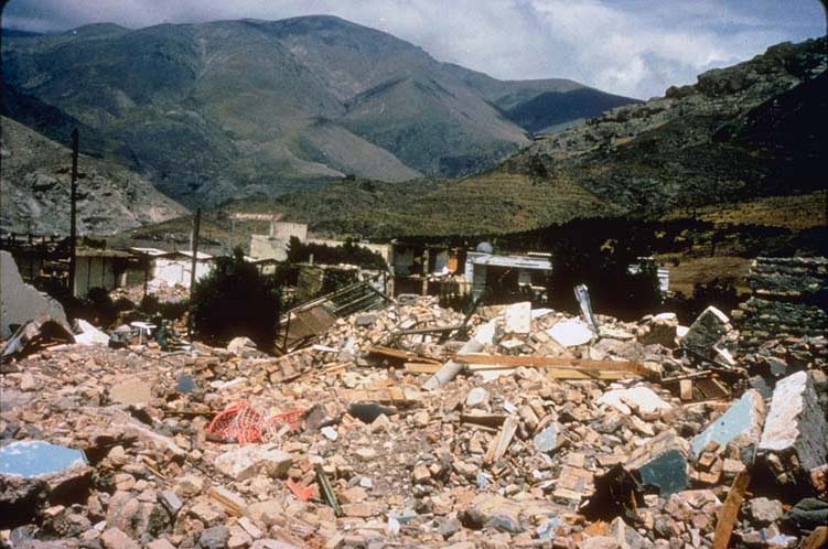
Charleston (1886): The 1886 earthquake in Charleston South Carolina was a moment magnitude 7.0, with a Mercalli intensity of X, caused significant ground motion, and killed at least 60 people. This intraplate earthquake was likely associated with ancient faults created during the breakup of Pangea. The earthquake caused significant liquefaction. Scientists estimate the recurrence of destructive earthquakes in this area with an interval of approximately 1500 to 1800 years.
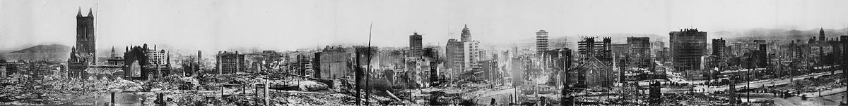
Great San Francisco earthquake and eire (1906): On April 18, 1906, a large earthquake, with an estimated moment magnitude of 7.8 and MMI of X, occurred along the San Andreas Fault near San Francisco California. There were multiple aftershocks followed by devastating fires, resulting in about 80% of the city being destroyed. Geologists G.K. Gilbert and Richard L. Humphrey, working independently, arrived the day following the earthquake and took measurements and photographs.
Alaska (1964): The 1964 Alaska earthquake, moment magnitude 9.2, was one of the most powerful earthquakes ever recorded. The earthquake originated in a megathrust fault along the Aleutian subduction zone. The earthquake caused large areas of land subsidence and uplift, as well as significant mass wasting.
Video from the USGS about the 1964 Alaska earthquake.

Video 9.18: The 1964 Alaska earthquake.
If you are using an offline version of this text, access this YouTube video via the QR code.
Loma Prieta (1989): The Loma Prieta, California, earthquake was created by movement along the San Andreas Fault. The moment magnitude 6.9 earthquake was followed by a magnitude 5.2 aftershock. It caused 63 deaths, buckled portions of the several freeways, and collapsed part of the San Francisco-Oakland Bay Bridge.
This video shows how shaking propagated across the Bay Area during the 1989 Loma Prieta earthquake.

Video 9.19: How shaking propagated across the Bay Area during the 1989 Loma Prieta earthquake.
If you are using an offline version of this text, access this YouTube video via the QR code.
This video shows destruction caused by the 1989 Loma Prieta earthquake.

Video 9.20: Destruction caused by the 1989 Loma Prieta earthquake.
If you are using an offline version of this text, access this YouTube video via the QR code.
9.9.2 Global Earthquakes
Many of history’s largest earthquakes occurred in megathrust zones, such as the Cascadia Subduction Zone (Washington and Oregon coasts) and Mt. Rainier (Washington).
Shaanxi, China (1556): On January 23, 1556 an earthquake of an approximate moment magnitude 8 hit central China, killing approximately 830,000 people in what is considered the most deadly earthquake in history. The high death toll was attributed to the collapse of cave dwellings (yaodong) built in loess deposits, which are large banks of windblown, compacted sediment (see chapter 5). Earthquakes in this are region are believed to have a recurrence interval of 1000 years.
Lisbon, Portugal (1755): On November 1, 1755 an earthquake with an estimated moment magnitude range of 8–9 struck Lisbon, Portugal, killing between 10,000 to 17,400 people. The earthquake was followed by a tsunami, which brought the total death toll to between 30,000-70,000 people.
Valdivia, Chile (1960): The May 22, 1960 earthquake was the most powerful earthquake ever measured, with a moment magnitude 9.4–9.6 and lasting an estimated 10 minutes. It triggered tsunamis that destroyed houses across the Pacific Ocean in Japan and Hawaii and caused vents to erupt on the Puyehue-Cordón Caulle (Chile).
Video describing the tsunami produced by the 1960 Chili earthquake.

Video 9.21: Tsunami produced by the 1960 Chili earthquake.
If you are using an offline version of this text, access this YouTube video via the QR code.
Tangshan, China (1976): Just before 4 a.m. (Beijing time) on July 28, 1976 a moment magnitude 7.8 earthquake struck Tangshan (Hebei Province), China, and killed more than 240,000 people. The high death-toll is attributed to people still being asleep or at home and most buildings being made of unreinforced masonry.
Sumatra, Indonesia (2004): On December 26, 2004, slippage of the Sunda megathrust fault generated a moment magnitude 9.0–9.3 earthquake off the coast of Sumatra, Indonesia. This megathrust fault is created by the Australia plate subducting below the Sunda plate in the Indian Ocean. The resultant tsunamis created massive waves as tall as 24 m (79 ft) when they reached the shore and killed more than an estimated 200,000 people along the Indian Ocean coastline.
Haiti (2010): The moment magnitude 7 earthquake that occurred on January 12, 2010, was followed by many aftershocks of magnitude 4.5 or higher. More than 200,000 people are estimated to have died as result of the earthquake. The widespread infrastructure damage and crowded conditions contributed to a cholera outbreak, which is estimated to have caused thousands more deaths.
Tōhoku, Japan (2011): Because most Japanese buildings are designed to tolerate earthquakes, the moment magnitude 9.0 earthquake on March 11, 2011, was not as destructive as the tsunami it created. The tsunami caused more than 15,000 deaths and tens of billions of dollars in damage, including the destructive meltdown of the Fukushima nuclear power plant.

Take this quiz to check your comprehension of this section.
If you are using an offline version of this text, access the quiz for section 9.9 via the QR code.
Summary
Geologic stress, applied force, comes in three types: tension, shear, and compression. Strain is produced by stress and produces three types of deformation: elastic, ductile, and brittle. Geological maps are two-dimensional representations of surface formations which are the surface expression of three-dimensional geologic structures in the subsurface. The map symbol called strike and dip or rock attitude indicates the orientation of rock strata with reference to north-south and horizontal. Folded rock layers are categorized by the orientation of their limbs, fold axes and axial planes. Faults result when stress forces exceed rock integrity and friction, leading to brittle deformation and breakage. The three major fault types are described by the movement of their fault blocks: normal, strike-slip, and reverse.
Earthquakes, or seismic activity, are caused by sudden brittle deformation accompanied by elastic rebound. The release of energy from an earthquake focus is generated as seismic waves. P and S waves travel through the Earth’s interior. When they strike the outer crust, they create surface waves. Human activities, such as mining and nuclear detonations, can also cause seismic activity. Seismographs measure the energy released by an earthquake using a logarithmic scale of magnitude units; the Moment Magnitude Scale has replaced the original Richter Scale. Earthquake intensity is the perceived effects of ground shaking and physical damage. The location of earthquake foci is determined from triangulation readings from multiple seismographs.
Earthquake rays passing through rocks of the Earth’s interior and measured at the seismographs of the worldwide Seismic Network allow 3-D imaging of buried rock masses as seismic tomographs.
Earthquakes are associated with plate tectonics. They usually occur around the active plate boundaries, including zones of subduction, collision, and transform and divergent boundaries. Areas of intraplate earthquakes also occur. The damage caused by earthquakes depends on a number of factors, including magnitude, location and direction, local conditions, building materials, intensity and duration, and resonance. In addition to damage directly caused by ground shaking, secondary earthquake hazards include liquefaction, tsunamis, landslides, seiches, and elevation changes.

Take this quiz to check your comprehension of this chapter.
If you are using an offline version of this text, access the quiz for chapter 9 via the QR code.
URLs Linked Within This Chapter
UGS geologic map viewer: https://geology.utah.gov/apps/intgeomap/
AAPG wiki: https://wiki.aapg.org/Cross_section
USGS Earthquakes Hazards Program: https://earthquake.usgs.gov/earthquakes/map/?extent=27.60567,-132.97852&extent=51.91717,-97.25098&range=week&magnitude=all&listOnlyShown=true&timeZone=utc&settings=true
Raleigh waves: Propagation of Seismic Waves: Rayleigh waves. [Video: 0:15] https://www.youtube.com/watch?v=6yXgfYHAS7c
Love waves: Propagation of Seismic Waves: Love waves. [Video: 0:15] https://www.youtube.com/watch?v=t7wJu0Kts7w
Blog.Wolfram.com: https://blog.wolfram.com/
International Registry of Seismograph Stations: http://www.isc.ac.uk/registries/
Global Seismic Network: https://www.usgs.gov/programs/earthquake-hazards/gsn-global-seismographic-network
USArray: http://www.usarray.org/
Comprehensive Nuclear Test Ban Treaty Organization: https://www.ctbto.org/
Fix the Bricks: https://www.slc.gov/em/fix-the-bricks
Text References
- Christenson, G.E., 1995, The September 2, 1992 ML 5.8 St. George earthquake, Washington County, Utah: Utah Geological Survey Circular 88, 48 p.
- Coleman, J.L., and Cahan, S.M., 2012, Preliminary catalog of the sedimentary basins of the United States: U.S. Geological Survey Open-File Report 1111, 27 p.
- Earle, S., 2015, Physical geology OER textbook: BC Campus OpenEd.
- Feldman, J., 2012, When the Mississippi Ran Backwards: Empire, Intrigue, Murder, and the New Madrid Earthquakes of 1811 and 1812: Free Press, 320 p.
- Fuller, M.L., 1912, The New Madrid earthquake: Central United States Earthquake Consortium Bulletin 494, 129 p.
- Gilbert, G.K., and Dutton, C.E., 1877, Report on the geology of the Henry Mountains: Washington, U.S. Government Printing Office, 160 p.
- Hildenbrand, T.G., and Hendricks, J.D., 1995, Geophysical setting of the Reelfoot rift and relations between rift structures and the New Madrid seismic zone: U.S. Geological Survey Professional Paper 1538-E, 36 p.
- Means, W.D., 1976, Stress and Strain – Basic Concepts of Continuum Mechanics: Berlin, Springe, 273 p.
- Ressetar, R. (Ed.), 2013, The San Rafael Swell and Henry Mountains Basin: geologic centerpiece of Utah: Utah Geological Association, Utah Geological Association, 250 p.
- Satake, K., and Atwater, B.F., 2007, Long-Term Perspectives on Giant Earthquakes and Tsunamis at Subduction Zones: Annual Review of Earth and Planetary Sciences, v. 35, no. 1, p. 349–374., doi: 10.1146/annurev.earth.35.031306.140302.
- Talwani, P., and Cox, J., 1985, Paleoseismic evidence for recurrence of Earthquakes near Charleston, South Carolina: Science, v. 229, no. 4711, p. 379–381.
Figure References
Figure 9.1: Types of stress. Michael Kimberly, North Carolina State University via USGS. 2021. Public domain. https://www.usgs.gov/media/images/stresstypesgif
Figure 9.2: Different materials deform differently when stress is applied. Steven Earle. 2019. CC BY. Figure 12.1.1 from https://opentextbc.ca/physicalgeology2ed/chapter/12-1-stress-and-strain/
Figure 9.3: “Strike” and “dip” are words used to describe the orientation of rock layers with respect to North/South and horizontal. CrunchyRocks. 2018. CC BY 4.0. https://commons.wikimedia.org/wiki/File:Strike_and_dip_on_bedding.svg
Figure 9.4: Attitude symbol on geologic map (with compass directions for reference) showing strike of N30°E and dip of 45° to the SE. Kindred Grey. 2022. CC BY 4.0. Includes Compass Rose by NAPISAH from Noun Project (Noun Project license).
Figure 9.5: Model of anticline. Speleotherm. 2016. CC BY-SA 4.0. https://commons.wikimedia.org/wiki/File:Anticline.png
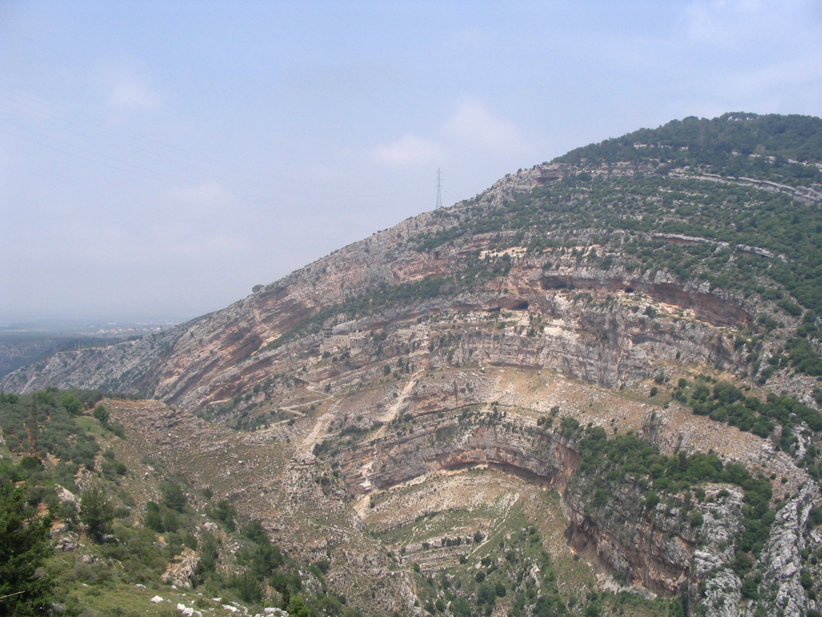
Figure 9.6: An Anticline near Bcharre, Lebanon. Not home. 2005. Public domain. https://commons.wikimedia.org/wiki/File:Anticline-lebanon.jpg
Figure 9.7: Monocline at Colorado National Monument. Anky-man. 2007. CC BY-SA 3.0. https://commons.wikimedia.org/wiki/File:Monocline.JPG
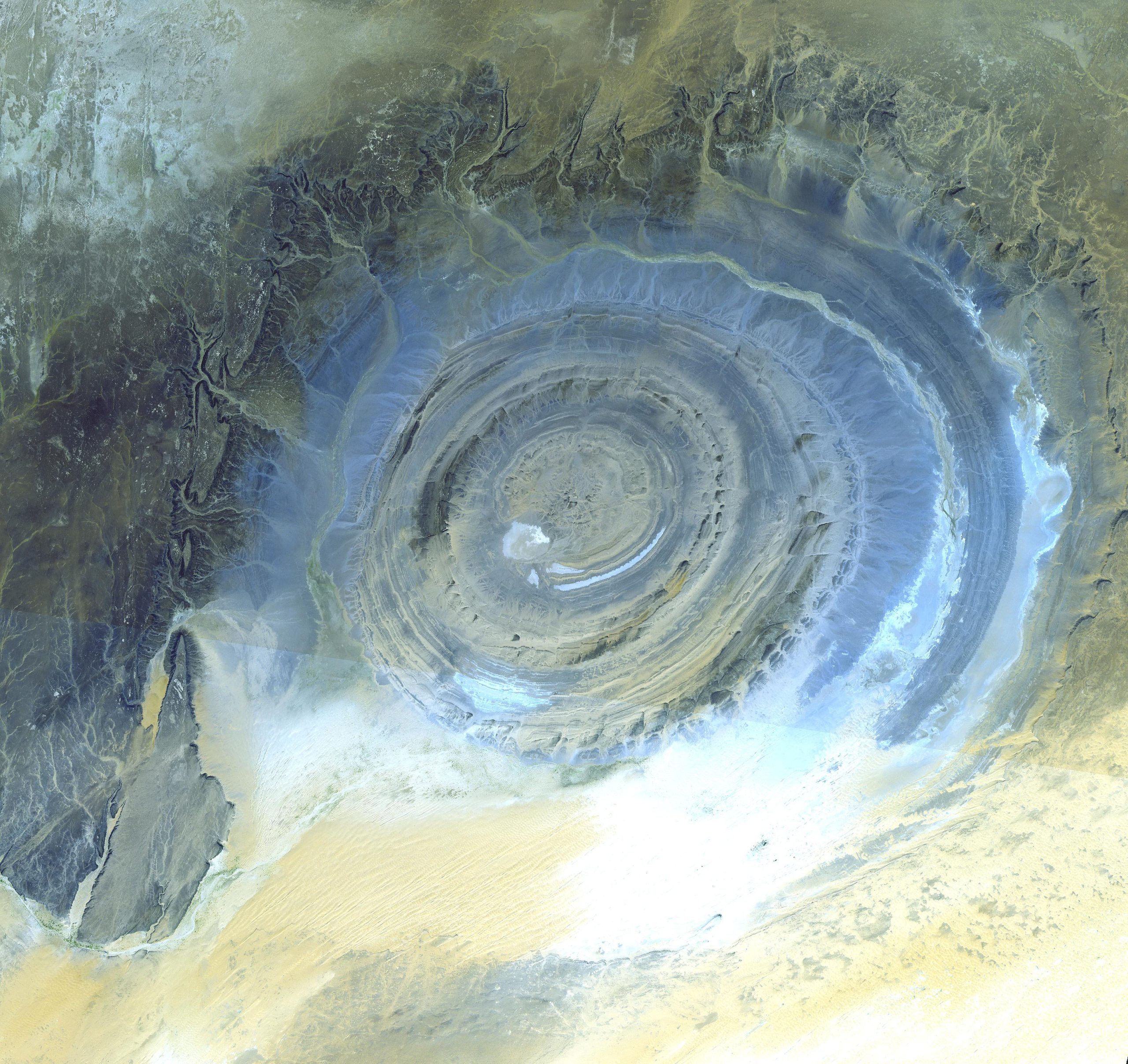
Figure 9.8: This prominent circular feature in the Sahara desert of Mauritania has attracted attention since the earliest space missions because it forms a conspicuous bull’s-eye in the otherwise rather featureless expanse of the desert. NASA/GSFC/MITI/ERSDAC/JAROS, and U.S./Japan ASTER Science Team. 2000. Public domain. https://commons.wikimedia.org/wiki/File:ASTER_Richat.jpg
Figure 9.9: The Denver Basin is an active sedimentary basin at the eastern extent of the Rocky Mountains. Daniel H. Knepper, Jr. (editor), US Geological Survey. 2002. Public domain. https://commons.wikimedia.org/wiki/File:Denver_Basin_Location_Map.png
Figure 9.10: Common terms used for normal faults. Kindred Grey. 2022. CC BY-SA 3.0. Includes Faults6 by Actualist, 2013 (CC BY-SA 3.0, https://commons.wikimedia.org/wiki/File:Faults6.png).
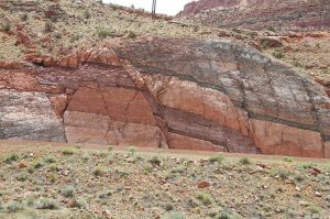
Figure 9.11: Example of a normal fault in an outcrop of the Pennsylvanian Honaker Trail Formation near Moab, Utah. James St. John. 2007. CC BY 2.0. https://commons.wikimedia.org/wiki/File:Faults_in_Moenkopi_Formation_Moab_Canyon_Utah_USA_01.jpg
Figure 9.12: Faulting that occurs in the crust under tensional stress. USGS; adapted by Gregors. 2011. Public domain. https://commons.wikimedia.org/wiki/File:Fault-Horst-Graben.svg
Figure 9.13: Simplified block diagram of a reverse fault. Kindred Grey. 2022. CC BY-SA 3.0. Includes Faults6 by Actualist, 2013 (CC BY-SA 3.0, https://commons.wikimedia.org/wiki/File:Faults6.png).
Figure 9.14: Terminology of thrust faults (low-angle reverse faults). Woudloper. 2006. Public domain. https://commons.wikimedia.org/wiki/File:Thrust_system_en.jpg
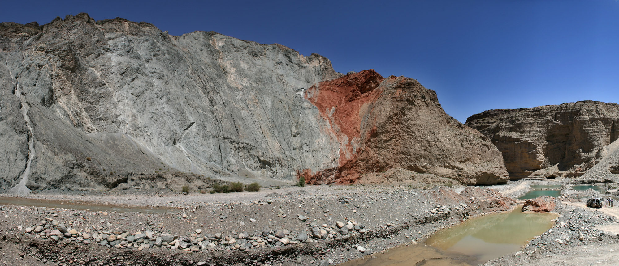
Figure 9.15: Thrust fault in the North Qilian Mountains (Qilian Shan). Jide. 2006. CC BY-SA 3.0. https://commons.wikimedia.org/wiki/File:Thrust_fault_Qilian_Shan.jpg
Figure 9.16: Flower structures created by strike-slip faults. Mikenorton. 2009. CC BY-SA 3.0. https://commons.wikimedia.org/wiki/File:Flowerstructure1.png
Figure 9.17: Process of elastic rebound: a) Undeformed state, b) accumulation of elastic strain, and c) brittle failure and release of elastic strain. Steven Earle. Unknown date. CC BY 4.0. Figure 11.2 from https://open.maricopa.edu/physicalgeology/chapter/11-1-what-is-an-earthquake/
Figure 9.18: The hypocenter is the point along the fault plane in the subsurface from which seismic energy emanates. Derived from original work by Sam Hocevar. 2014. CC BY-SA 1.0. https://commons.wikimedia.org/wiki/File:Epicenter_Diagram.svg
Figure 9.19: Example of constructive and destructive interference; note red line representing the results of interference. Lookangmany thanks to author of original simulation = Wolfgang Christian and Francisco Esquembre author of Easy Java Simulation = Francisco Esquembre. 2015. CC BY-SA 4.0. https://www.wikiwand.com/en/Wave_interference#Media/File:Waventerference.gif
Figure 9.20: P-waves are compressional. Christophe Dang Ngoc Chan. 2006. CC BY-SA 3.0. https://commons.wikimedia.org/wiki/File:Onde_compression_impulsion_1d_30_petit.gif
Figure 9.21: S waves are shear. Christophe Dang Ngoc Chan. 2006. CC BY-SA 3.0. https://commons.wikimedia.org/wiki/File:Onde_cisaillement_impulsion_1d_30_petit.gif
Figure 9.22: Frequency of earthquakes in the central United States. USGS. 2019. Public domain. https://commons.wikimedia.org/wiki/File:Cumulative_induced_seismicity.png
Figure 9.23: A seismogram showing the arrivals of the P, S, and surface waves. Kindred Grey. 2022. CC BY 4.0. Adapted from USGS (Public domain, https://www.usgs.gov/media/images/seismic-wave-showing-p-wave-and-s-wave-initiation).
Figure 9.24: Global network of seismic stations. USGS. 2022. Public domain. https://www.usgs.gov/media/images/global-seismographic-network-gsn-stations
Figure 9.25: Speed of seismic waves with depth in the earth. Brews ohare. 2010. CC BY-SA 3.0. https://commons.wikimedia.org/wiki/File:Speeds_of_seismic_waves.PNG
Figure 9.26: Simplified and interpreted P- and S-wave velocity variations in the mantle across southern North America showing the subducted Farallon Plate. Oilfieldvegetarian. 2016. CC BY-SA 4.0. https://commons.wikimedia.org/wiki/File:FarallonTomoSlice.png
Figure 9.27: Tomographic image of the Farallon plate in the mantle below North America. Stuart A. Snodgrass and Hans-Peter Bunge via NASA. 2002. Public domain. https://commons.wikimedia.org/wiki/File:Farallon_Plate.jpg
Figure 9.28: Example of a shake map. USGS. 2012. Public domain. https://en.wikipedia.org/wiki/File:USGS_Shakemap_-_1979_Imperial_Valley_earthquake.jpg
Figure 9.29: Example of devastation on unreinforced masonry by seismic motion. M. Mehrain, Dames and Moore via NOAA/NGDC. 2012. Public domain. https://commons.wikimedia.org/wiki/File:Collapse_of_Unreinforced_Masonry_Buildings,_Iran_(Persia)_-_1990_Manjil_Roudbar_Earthquake.jpg
Figure 9.30: Fault trench near Teton Fault. Jaime Delano via USGS. 2017. Public domain. https://www.usgs.gov/media/images/teton-fault-4
Figure 9.31: High density of earthquakes in the New Madrid seismic zone. Kbh3rd. 2011. CC BY-SA 3.0. https://commons.wikimedia.org/wiki/File:New_Madrid_Seismic_Zone_activity_1974-2011.svg
Figure 9.32: Buildings toppled from liquefaction during a 7.5 magnitude earthquake in Japan. Ungtss. 1964. Public domain. https://commons.wikimedia.org/wiki/File:Liquefaction_at_Niigata.JPG
Figure 9.33: As the ocean depth becomes shallower, the wave slows down and pile up on top of itself, making large, high-amplitude waves. Régis Lachaume. 2005. CC BY-SA 3.0. https://commons.wikimedia.org/wiki/File:Propagation_du_tsunami_en_profondeur_variable.gif
Figure 9.34: Schoolhouse in Thistle, Utah destroyed by a landslide. Jenny Bauman. 2006. CC BY-SA 2.0. https://commons.wikimedia.org/wiki/File:Thistle-School_house.jpg
Figure 9.35: Remains of San Francisco after the 1906 earthquake and fire. Lester C. Guernsey. 1906. Public domain. https://commons.wikimedia.org/wiki/File:San_Francisco_1906_earthquake_Panoramic_View.jpg
Force applied to an object, typically dealing with forces within the Earth.
The deformation that results from application of a stress.
A property of solids in which a force applied to an object causes the object to fracture, break, or snap. Most rocks, at low temperatures, are brittle.
A property of a solid, such that when a force is applied, the solid flows, stretches, or bends along with the force, instead of cracking or breaking. For example, many plastics are ductile.
A type of deformation that reverses when the stress is removed.
A measure of a geologic plane's orientation in 3-D space. Used for beds of rocks, faults, fold hinges, etc. Using the right hand rule, dip is perpendicular, and to the right 90° of the strike.
A measure of a plane's (maximum) angle with respect to horizontal, where a perfectly horizontal plane has a dip of zero and a vertical plane has a dip of 90°.
Discernible layers of rock, typically from a sedimentary rock.
A rock layer that has been bent in a ductile way instead of breaking (as with faulting).
Planar feature where two blocks of bedrock move past each other via earthquakes.
A theory of building energy that is released during an earthquake.
Energy that radiates from fault movement via earthquakes.
Instrument used to measure seismic energy.
A measure of earthquake strength. Scales include Richter and Moment.
A strain that occurs in a substance in which the item changes shape due to a stress.
Relating to the movement of plates of lithosphere.
Rocks that are formed from liquid rock, i.e. from volcanic processes.
A coherent body of intrusive rock (which formed underground) which is now at (or near) the surface.
A break within a rock that has no relative movement between the sides. Caused by cooling, pressure release, tectonic forces, etc.
Stress within an object that causes a side-to-side movement within an internal fabric or weakness.
A style of strain in which an object suddenly breaks, fractures, or otherwise fails in a different way than ductile deformation.
Stresses that pull objects apart into a larger surface area or volume; stretching forces.
Stresses that push objects together into a smaller surface area or volume; contracting forces.
A separation of light (felsic) and dark (mafic) minerals in higher grade metamorphic rocks like gneiss.
A bending, squishing, or stretching style of deformation where an object changes shape smoothly.
An amount of strain where the substance has a maximum amount of elastic deformation and switches to ductile deformation.
Empty space in a geologic material, either within sediments, or within rocks. Can be filled by air, water, or hydrocarbons.
The measure of the vibrational (kinetic) energy of a substance.
Non-directional pressure resulting from burial.
Pieces of rock that have been weathered and possibly eroded.
A very fine-grained rock with very thin layering (fissile).
General name of a felsic rock that is intrusive. Has more felsic minerals than mafic minerals.
An extensive, distinct, and mapped set of geologic layers.
A unit of the geologic time scale; smaller than an era, larger than an epoch. We are currently in the Quaternary period.
A specific layer of rock with identifiable properties.
Dividing two-dimensional line between the two sides of a fold.
Downward-facing fold, that has older rock in its core.
A U-shaped, upward-facing fold with younger rocks in its core.
A one-sided fold-like structure in which layers of rock warp upwards or downwards.
A rock up-warping of symmetrical anticlines.
A down-warped feature in the crust.
A dark liquid fossil fuel derived from petroleum.
A geologic circumstance (such as a fold, fault, change in lithology, etc.) which allows petroleum resources to collect.
Bottommost part of a wave.
A topographic high found away from the beach in deeper water, but still on the continental shelf. Typically, these are formed in tropical areas by organisms such as corals.
A dip-slip fault that has the hanging wall moving up with respect to the foot wall.
A local or regional depression which allows sediments to accumulate.
The act of the land surface down-warping, typically referred to when discussing sedimentation or with rapid groundwater removal.
The last period of the Paleozoic, 299-252 million years ago.
Adjective for a rock filled with fossils, most commonly with limestones.
A rock primarily made of sand.
A chemical or biochemical rock made of mainly calcite.
The outermost chemical layer of the Earth, defined by its low density and higher concentrations of lighter elements. The crust has two types: continental, which is the thick, more ductile, and lowest density, and oceanic, which is higher density, more brittle, and thinner.
Faulting that occurs with a vertical motion.
On a dipping fault, the side that is on top of the fault plane. Moves down in normal faulting, up in reverse faulting.
On a dipping fault, the part of the block that is below the fault. Moves down in normal faulting, up in reverse faulting.
An interconnected set of parts that combine and make up a whole.
Place where material is extracted from the Earth for human use.
A solid part of the lithosphere which moves as a unit, i.e. the entire plate generally moves the same direction at the same speed.
Place where fault movement cuts the surface of the Earth.
Amount of movement during a faulting event.
A polished surface of rock from fault movement, covered with grooves.
Place where two plates are moving apart, creating either a rift (continental lithosphere) or a mid-ocean ridge (oceanic lithosphere).
Term for the extensional tectonic province that extends from California’s Sierra Nevada Mountains in the west, to Utah’s Wasatch Mountains to the east, to southern Oregon and Idaho to the north, to northern Mexico to the south. Known as a wide rift, each graben (basin) is bounded by horsts (ranges).
A valley formed by normal faulting.
Uplifted mountain block caused by normal faulting.
A valley formed by normal faulting on just one side.
A dip-slip fault in which the hanging wall drops relative to the footwall, caused by extensional forces.
Middle chemical layer of the Earth, made of mainly iron and magnesium silicates. It is generally denser than the crust (except for older oceanic crust) and less dense than the core.
A low-angle reverse fault, common in mountain building.
The study of rock layers and their relationships to each other within a specific area.
Place where two plates come together, casing subduction or collision.
A process where an oceanic plate descends bellow a less dense plate, causing the removal of the plate from the surface. Subduction causes the largest earthquakes possible, as the subducting plate can lock as it goes down. Volcanism is also caused as the plate releases volatiles into the mantle, causing melting.
Term for faulting that occurs in subduction.
The thin, outer layer of the Earth which makes up the rocky bottom of the ocean basins. Oceanic crust is much thinner (but denser) than continental crust. Oceanic crust is made of rocks similar to basalt and as it cools, becomes more dense.
A feature with no internal structure, habit, or layering.
A series of waves produced from a sudden movement of the floor of a ocean basin (or large lake), caused by events such as earthquakes, volcanic eruptions, landslides, and bolide impacts.
Faulting that occurs with shear forces, typically on vertical fault plaines as two fault blocks slide past each other.
Place where two plates slide past each other, creating strike slip faults.
A divergent boundary within an oceanic plate, where new lithosphere and crust is created as the two plates spread apart. Mid-ocean ridge and spreading center are synonyms.
A strike-slip or transform motion in which the relative motion is to the left. As viewed across the fault, objects will move to the left.
Movement in a transform or strike-slip setting which is toward the right across the fault. As viewed across the fault, objects will move to the right.
A segment along a transform or strike-slip fault which has a compressional component, sometimes creating related thrust faulting and mountains.
A place along a transform or strike-slip fault with an extensional component, sometimes including normal faulting, basin formation, and volcanism.
A small area along a strike-slip or transform fault with branching structures of transpression/transtension, causing local hills or valleys.
Activities that occur within plates, away from plate boundaries.
An accepted scientific idea that explains a process using the best available information.
Initiation point of an earthquake or fault movement.
A slow and steady movement. Can occur as part of faults, mass wasting, and grain movement.
An earthquake that sometimes occurs before the larger mainshock.
Largest earthquake in an earthquake sequence.
Earthquake(s) that occur after the mainshock, usually decreasing in amount and magnitude over time.
The location at the surface directly above the focus of an earthquake, typically associated with strong damage.
Height or depth of a wave from the middle point.
The distance between any two repeating portions of a wave (e.g., two successive wave crests).
Seismic waves that travel through the Earth, mainly P waves and S waves.
Seismic waves that only move along the surface, mainly R waves and L waves.
The fastest seismic wave that occurs after an earthquake, compressional in nature.
Second-fastest seismic wave that has a shear motion.
Waves that change direction due to changing speeds, typically caused by a change in density of the medium.
Surface waves that have a side-to-side motion.
Surface waves that have an up and down motion.
The outer physical layer of the core, which is liquid. Movement within the outer core is believed to be responsible for Earth's magnetic field and flips of the magnetic field.
The innermost chemical layer of the Earth, made chiefly of iron and nickel. It has both liquid and solid components.
Earthquakes that occur due to human activity.
Gaseous fossil fuel derived from petroleum, mostly made of methane.
A process of injecting pressurized fluids into the ground to aid in hydrocarbon migration.
A magnitude scale based on calculation of the energy released in an earthquake.
A place where pressurized groundwater flows onto the surface.
A process of using 3D seismic arrays to get subsurface images.
Areas that have an unpredicted change in seismic data, indicating a change in properties.
The theory that the outer layer of the Earth (the lithosphere) is broken in several plates, and these plates move relative to one another, causing the major topographic features of Earth (e.g. mountains, oceans) and most earthquakes and volcanoes.
A reservoir of magma below a volcano.
Rising stationary magma, forming a succession of volcanism. This is reflected as islands on oceanic plates, and volcanic mountains or craters on land.
The layers of igneous, sedimentary, and metamorphic rocks that form the continents. Continental crust is much thicker than oceanic crust. Continental crust is defined as having higher concentrations of very light elements like K, Na, and Ca, and is the lowest density rocky layer of Earth. Its average composition is similar to granite.
A magnitude scale using the amplitude of shaking via a seismograph.
A qualitative earthquake scale, from I-XII, of the degree of shaking in an earthquake.
An observation which is based on non-numerical data. While these types of observations are not preferred, they can still be useful.
An observation which is based on numerical data. These observations are preferred because they can be used in calculations.
Rocks and minerals that change within the Earth are called metamorphic, changed by heat and pressure. Metamorphism is the name of the process.
Term for the underlying lithified rocks that make up the geologic record in an area. This term can sometimes refer to only the deeper, crystalline (non-layered) rocks.
Speed at which a wave travels past a fixed point.
An amplification of earthquake waves due to a structure of buildings or structures.
Average time between earthquakes calculated based on past earthquake records.
Place where lava is erupted at the surface.
When two continents crash, with no subduction (and thus little to no volcanism), since each continent is too buoyant. Many of the largest mountain ranges and broadest zones of seismic activity come from collisions.
Area of extended continental lithosphere, forming a depression. Rifts can be narrow (focused in one place) or broad (spread out over a large area with many faults).
A mechanical process which takes ore and separates it from gangue material.
Stress that has a strong directional component (unequal), typically creating elongated or flattened features.
Process of saturated sediments becoming internally weak (like quicksand) and destabilizing foundations.
A solution that has the maximum allowed dissolved component, and is unable to dissolve more.
Forces that hold a substance together.
General term for sudden material falling (sliding) down a slope due to gravity.
The part of the coastline which is directly related to water-land interaction, specifically the tidal zone and the range of wave base.
Top of a wave.
An event that causes a landslide event. Water is a common trigger.
A channelled body of water.
The most recent supercontinent, which formed over 300 million years ago and started breaking apart less than 200 million years ago. Africa and South America, as well as Europe and North America, bordered each other.
Any downhill movement of material, caused by gravity.
Wind-blown silt, mainly formed from glacial processes.
The entire area which is related to land-sea interactions.
