7 Geologic Time
Learning Objectives
By the end of this chapter, students should be able to:
- Explain the difference between relative time and numeric time.
- Describe the five principles of stratigraphy.
- Apply relative dating principles to a block diagram and interpret the sequence of geologic events.
- Define an isotope, and explain alpha decay, beta decay, and electron capture as mechanisms of radioactive decay.
- Describe how radioisotopic dating is accomplished and list the four key isotopes used.
- Explain how carbon-14 forms in the atmosphere and how it is used in dating recent events.
- Explain how scientists know the numeric age of the Earth and other events in Earth history.
- Explain how sedimentary sequences can be dated using radioisotopes and other techniques.
- Define a fossil and describe types of fossils preservation.
- Outline how natural selection takes place as a mechanism of evolution.
- Describe stratigraphic correlation.
- List the eons, eras, and periods of the geologic time scale and explain the purpose behind the divisions.
- Explain the relationship between time units and corresponding rock units—chronostratigraphy versus lithostratigraphy.

The geologic time scale and basic outline of Earth’s history were worked out long before we had any scientific means of assigning numerical age units, like years, to events of Earth history. Working out Earth’s history depended on realizing some key principles of relative time. Nicolas Steno (1638-1686) introduced basic principles of stratigraphy, the study of layered rocks, in 1669. William Smith (1769-1839), working with the strata of English coal mines, noticed that strata and their sequence were consistent throughout the region. Eventually he produced the first national geologic map of Britain, becoming known as “the Father of English Geology.” Nineteenth-century scientists developed a relative time scale using Steno’s principles, with names derived from the characteristics of the rocks in those areas. The figure of this geologic time scale shows the names of the units and subunits. Using this time scale, geologists can place all events of Earth history in order without ever knowing their numerical ages. The specific events within Earth history are discussed in chapter 8.
7.1 Relative Dating
Relative dating is the process of determining if one rock or geologic event is older or younger than another, without knowing their specific ages—i.e., how many years ago the object was formed. The principles of relative time are simple, even obvious now, but were not generally accepted by scholars until the scientific revolution of the 17th and 18th centuries. James Hutton (see chapter 1) realized geologic processes are slow and his ideas on uniformitarianism (i.e., “the present is the key to the past”) provided a basis for interpreting rocks of the Earth using scientific principles.
7.1.1 Relative Dating Principles
Stratigraphy is the study of layered sedimentary rocks. This section discusses principles of relative time used in all of geology, but are especially useful in stratigraphy.
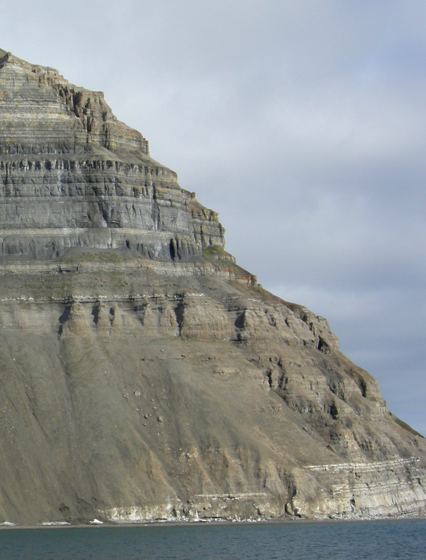
Principle of Superposition: In an otherwise undisturbed sequence of sedimentary strata, or rock layers, the layers on the bottom are the oldest and layers above them are younger.
Principle of Original Horizontality: Layers of rocks deposited from above, such as sediments and lava flows, are originally laid down horizontally. The exception to this principle is at the margins of basins, where the strata can slope slightly downward into the basin.
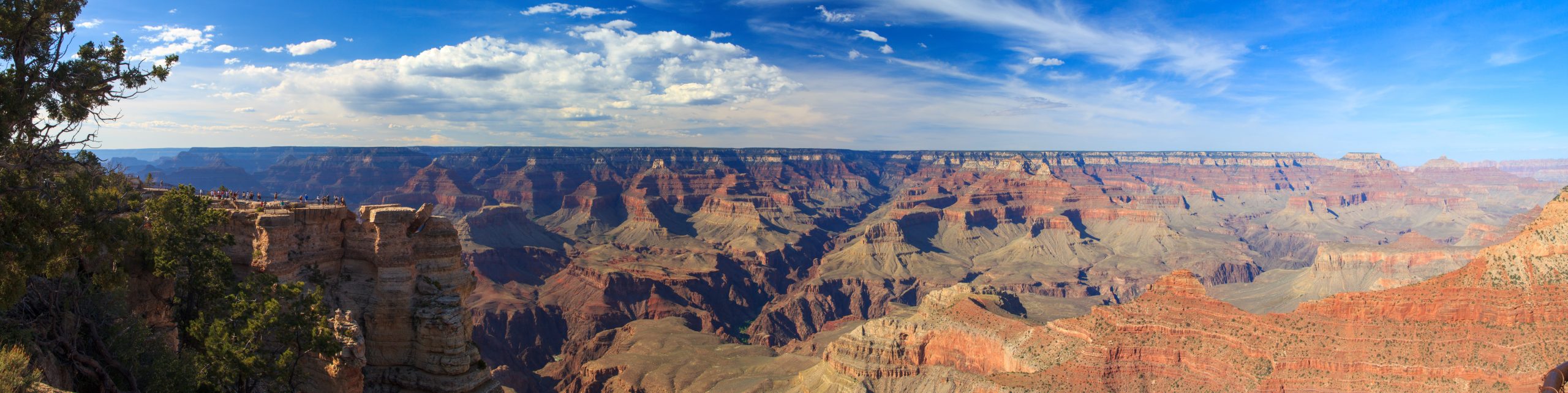
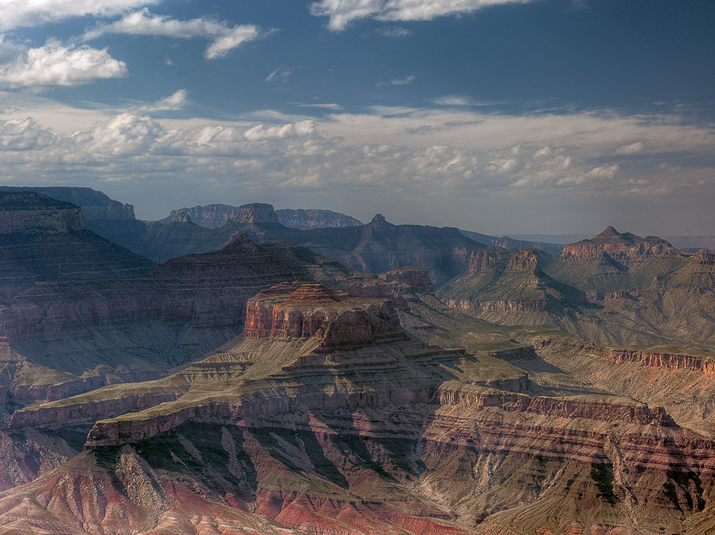
Principle of Lateral Continuity: Within the depositional basin, strata are continuous in all directions until they thin out at the edge of that basin. Of course, all strata eventually end, either by hitting a geographic barrier, such as a ridge, or when the depositional process extends too far from its source, either a sediment source or a volcano. Strata that are cut by a canyon later remain continuous on either side of the canyon.
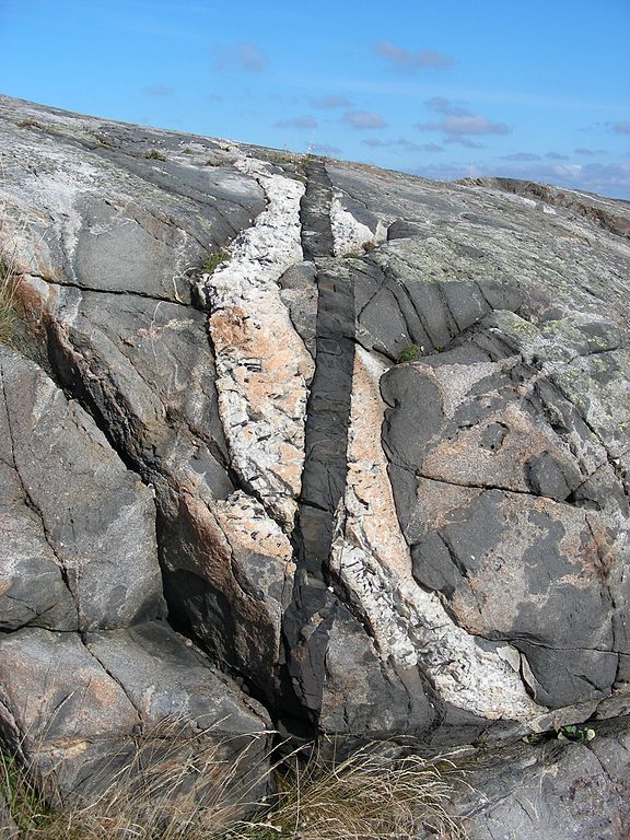
Principle of Cross-Cutting Relationships: Deformation events like folds, faults and igneous intrusions that cut across rocks are younger than the rocks they cut across.
Principle of Inclusions: When one rock formation contains pieces or inclusions of another rock, the included rock is older than the host rock.
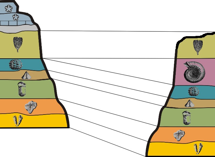
Principle of Fossil Succession: Evolution has produced a succession of unique fossils that correlate to the units of the geologic time scale. Assemblages of fossils contained in strata are unique to the time they lived, and can be used to correlate rocks of the same age across a wide geographic distribution. Assemblages of fossils refers to groups of several unique fossils occurring together.
7.1.2 Grand Canyon Example
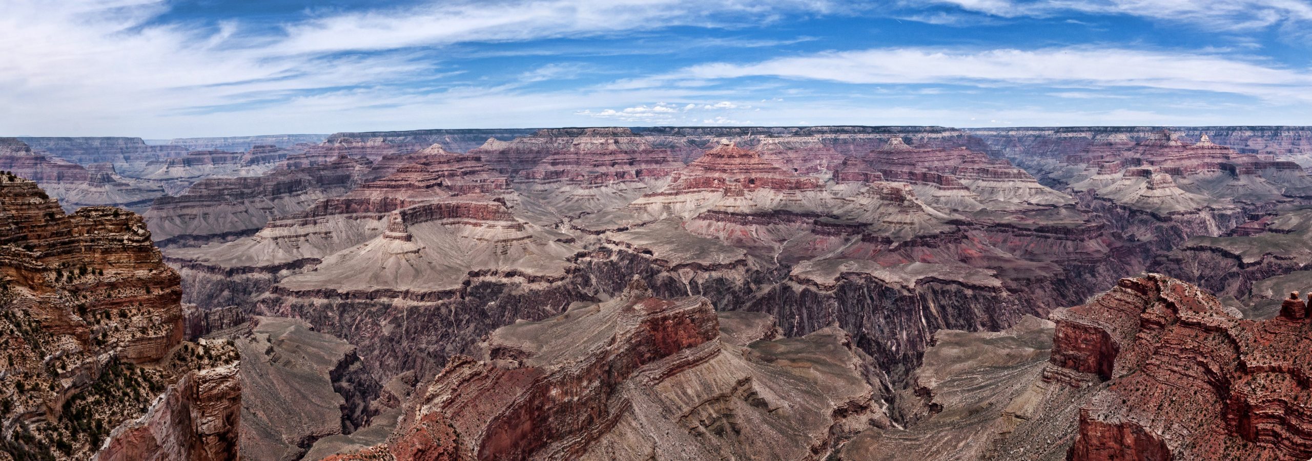
The Grand Canyon of Arizona illustrates the stratigraphic principles. The photo shows layers of rock on top of one another in order, from the oldest at the bottom to the youngest at the top, based on the principle of superposition. The predominant white layer just below the canyon rim is the Coconino Sandstone. This layer is laterally continuous, even though the intervening canyon separates its outcrops. The rock layers exhibit the principle of lateral continuity, as they are found on both sides of the Grand Canyon which has been carved by the Colorado River.
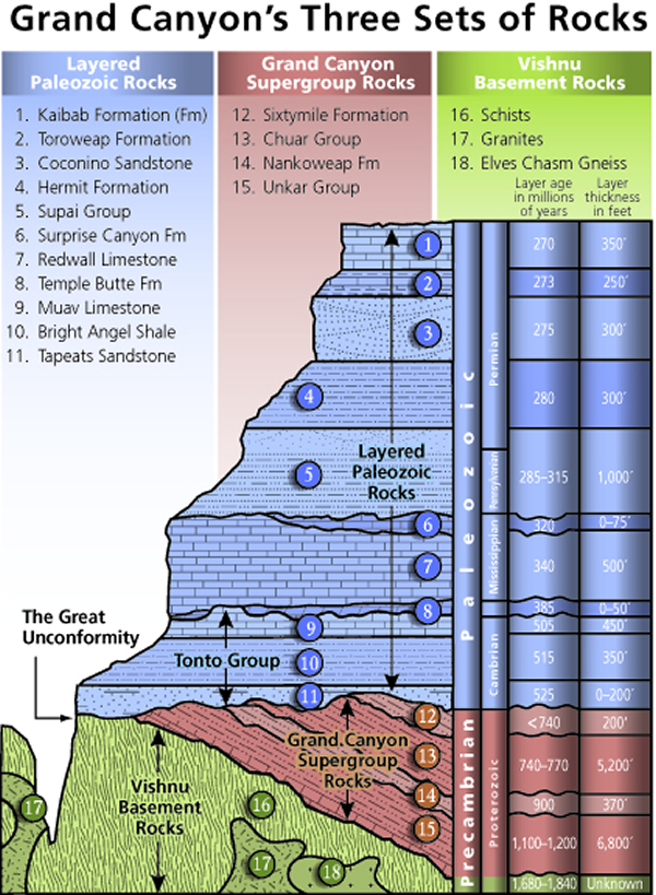
The diagram called “Grand Canyon’s Three Sets of Rocks” shows a cross-section of the rocks exposed on the walls of the Grand Canyon, illustrating the principle of cross-cutting relationships, superposition, and original horizontality. In the lowest parts of the Grand Canyon are the oldest sedimentary formations, with igneous and metamorphic rocks at the bottom. The principle of cross-cutting relationships shows the sequence of these events. The metamorphic schist (#16) is the oldest rock formation and the cross-cutting granite intrusion (#17) is younger. As seen in the figure, the other layers on the walls of the Grand Canyon are numbered in reverse order with #15 being the oldest and #1 the youngest. This illustrates the principle of superposition. The Grand Canyon region lies in Colorado Plateau, which is characterized by horizontal or nearly horizontal strata, which follows the principle of original horizontality. These rock strata have been barely disturbed from their original deposition, except by a broad regional uplift.
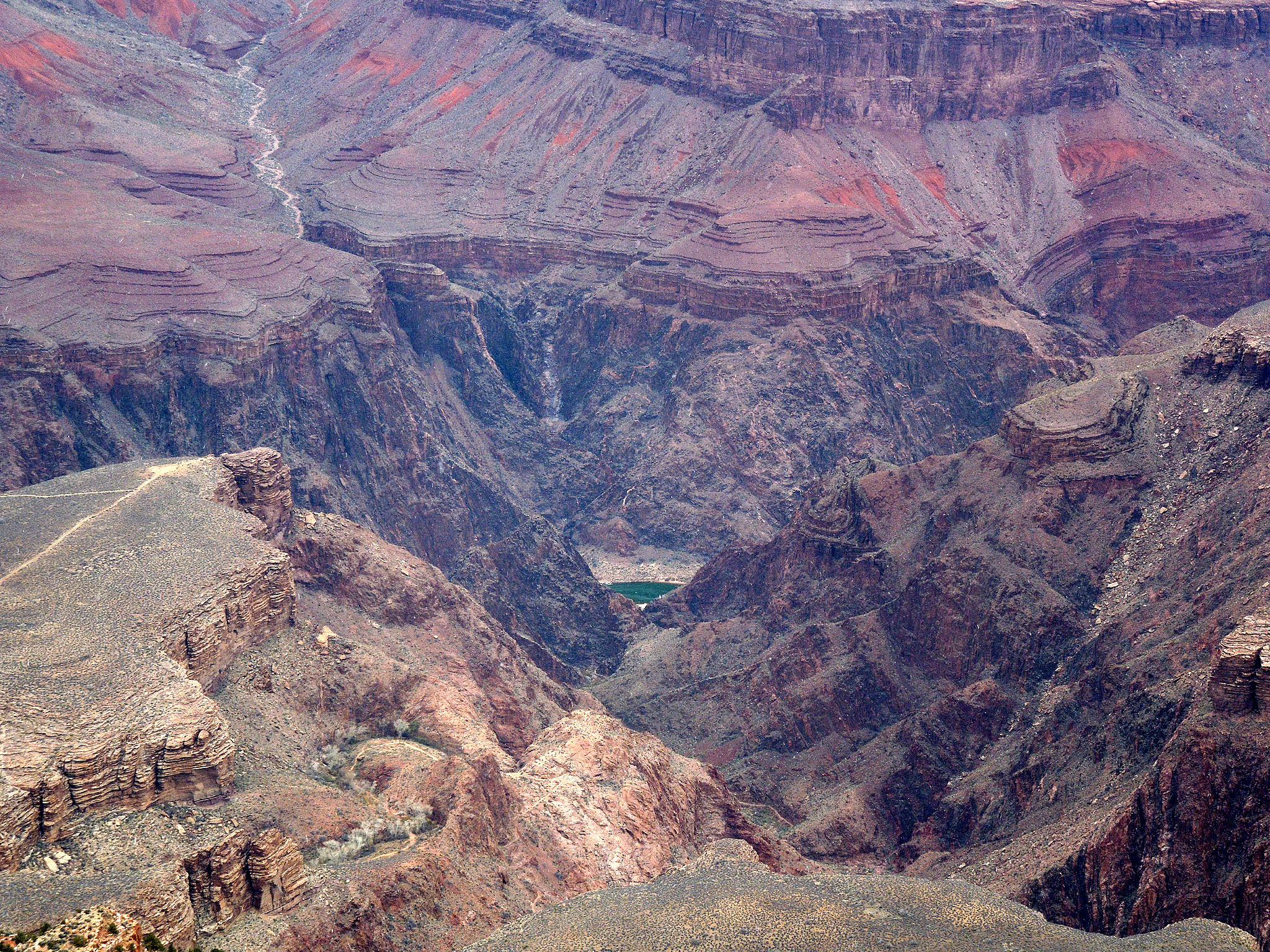
The photo of the Grand Canyon here show strata that were originally deposited in a flat layer on top of older igneous and metamorphic “basement” rocks, per the original horizontality principle. Because the formation of the basement rocks and the deposition of the overlying strata is not continuous but broken by events of metamorphism, intrusion, and erosion, the contact between the strata and the older basement is termed an unconformity. An unconformity represents a period during which deposition did not occur or erosion removed rock that had been deposited, so there are no rocks that represent events of Earth history during that span of time at that place. Unconformities appear in cross sections and stratigraphic columns as wavy lines between formations. Unconformities are discussed in the next section.
7.1.3 Unconformities
There are three types of unconformities, nonconformity, disconformity, and angular unconformity. A nonconformity occurs when sedimentary rock is deposited on top of igneous and metamorphic rocks as is the case with the contact between the strata and basement rocks at the bottom of the Grand Canyon.
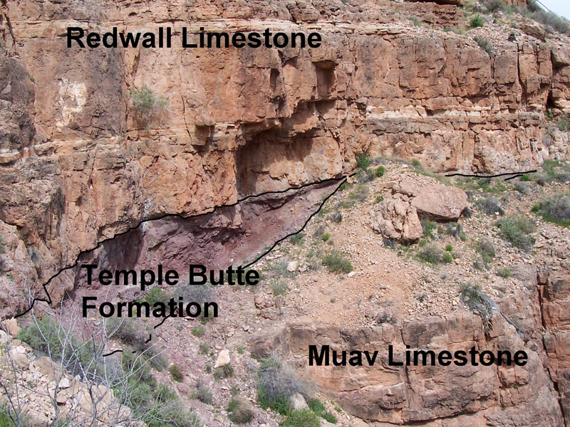
The strata in the Grand Canyon represent alternating marine transgressions and regressions where sea level rose and fell over millions of years. When the sea level was high marine strata formed. When sea-level fell, the land was exposed to erosion creating an unconformity. In the Grand Canyon cross-section, this erosion is shown as heavy wavy lines between the various numbered strata. This is a type of unconformity called a disconformity, where either non-deposition or erosion took place. In other words, layers of rock that could have been present, are absent. The time that could have been represented by such layers is instead represented by the disconformity. Disconformities are unconformities that occur between parallel layers of strata indicating either a period of no deposition or erosion.
The Phanerozoic strata in most of the Grand Canyon are horizontal. However, near the bottom horizontal strata overlie tilted strata. This is known as the Great Unconformity and is an example of an angular unconformity. The lower strata were tilted by tectonic processes that disturbed their original horizontality and caused the strata to be eroded. Later, horizontal strata were deposited on top of the tilted strata creating the angular unconformity.
Here are three graphical illustrations of the three types of unconformity.
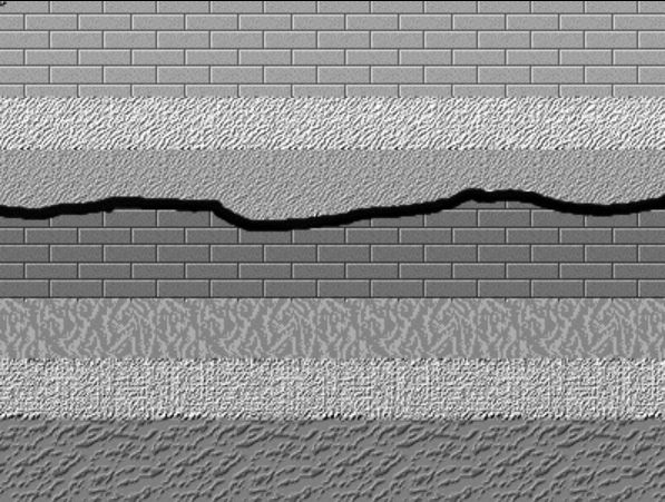
Disconformity, where is a break or stratigraphic absence between strata in an otherwise parallel sequence of strata.
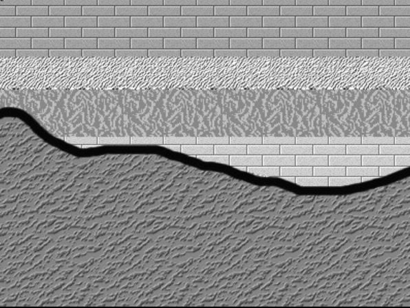
Nonconformity, where sedimentary strata are deposited on crystalline (igneous or metamorphic) rocks.
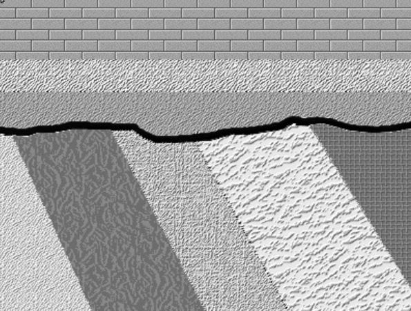
Angular unconformity, where sedimentary strata are deposited on a terrain developed on sedimentary strata that have been deformed by tilting, folding, and/or faulting. so that they are no longer horizontal.
7.1.3 Applying Relative Dating Principles
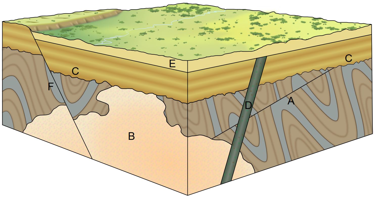
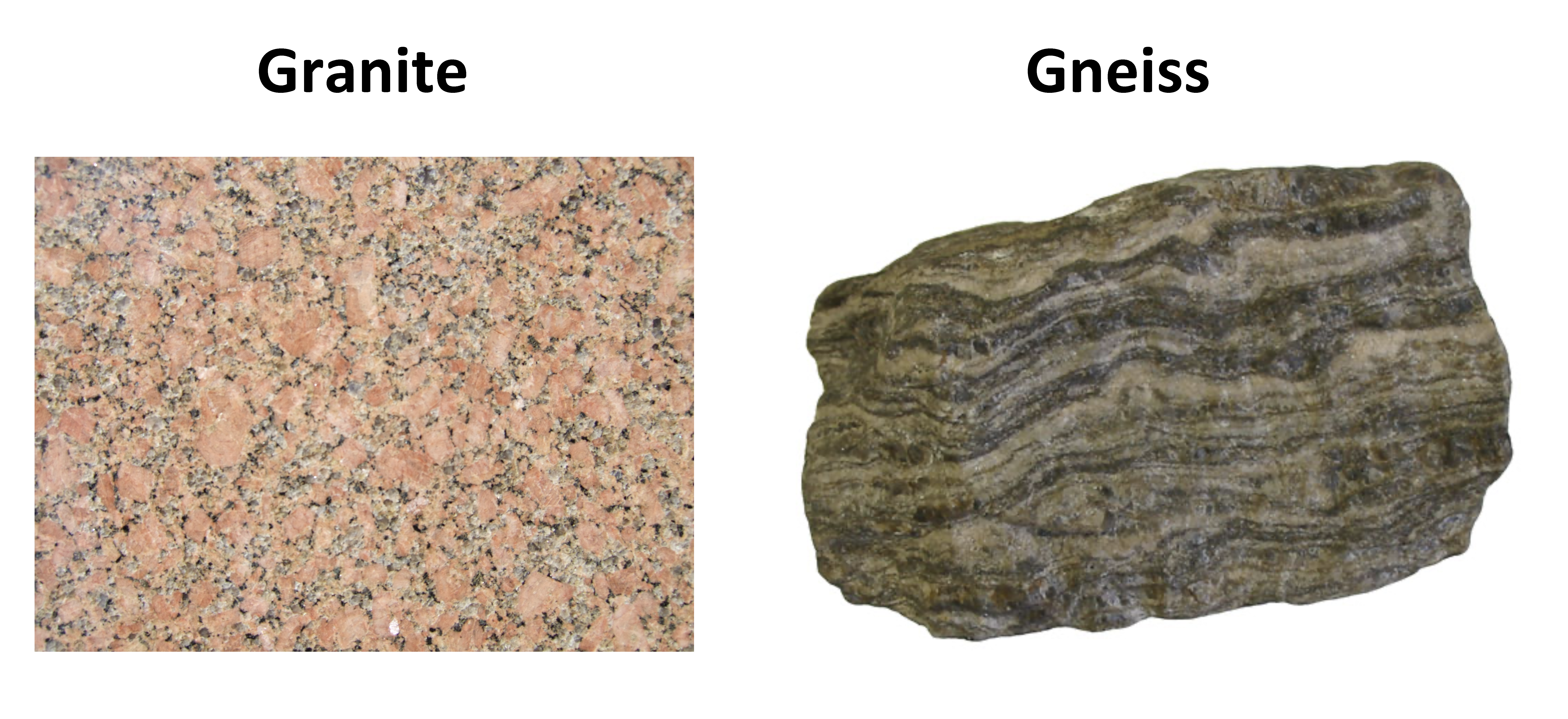
In the block diagram, the sequence of geological events can be determined by using the relative-dating principles and known properties of igneous, sedimentary, metamorphic rock (see chapter 4, chapter 5, and chapter 6). The sequence begins with the folded metamorphic gneiss on the bottom. Next, the gneiss is cut and displaced by the fault labeled A. Both the gneiss and fault A are cut by the igneous granitic intrusion called batholith B; its irregular outline suggests it is an igneous granitic intrusion emplaced as magma into the gneiss. Since batholith B cuts both the gneiss and fault A, batholith B is younger than the other two rock formations. Next, the gneiss, fault A, and batholith B were eroded forming a nonconformity as shown with the wavy line. This unconformity was actually an ancient landscape surface on which sedimentary rock C was subsequently deposited perhaps by a marine transgression. Next, igneous basaltic dike D cut through all rocks except sedimentary rock E. This shows that there is a disconformity between sedimentary rocks C and E. The top of dike D is level with the top of layer C, which establishes that erosion flattened the landscape prior to the deposition of layer E, creating a disconformity between rocks D and E. Fault F cuts across all of the older rocks B, C and E, producing a fault scarp, which is the low ridge on the upper-left side of the diagram. The final events affecting this area are current erosion processes working on the land surface, rounding off the edge of the fault scarp, and producing the modern landscape at the top of the diagram.

Take this quiz to check your comprehension of this section.
If you are using an offline version of this text, access the quiz for section 7.1 via the QR code.
7.2 Absolute Dating
Relative time allows scientists to tell the story of Earth events, but does not provide specific numeric ages, and thus, the rate at which geologic processes operate. Based on Hutton’s principle of uniformitarianism (see chapter 1), early geologists surmised geological processes work slowly and the Earth is very old. Relative dating principles was how scientists interpreted Earth history until the end of the 19th Century. Because science advances as technology advances, the discovery of radioactivity in the late 1800s provided scientists with a new scientific tool called radioisotopic dating. Using this new technology, they could assign specific time units, in this case years, to mineral grains within a rock. These numerical values are not dependent on comparisons with other rocks such as with relative dating, so this dating method is called absolute dating. There are several types of absolute dating discussed in this section but radioisotopic dating is the most common and therefore is the focus on this section.
7.2.1 Radioactive Decay
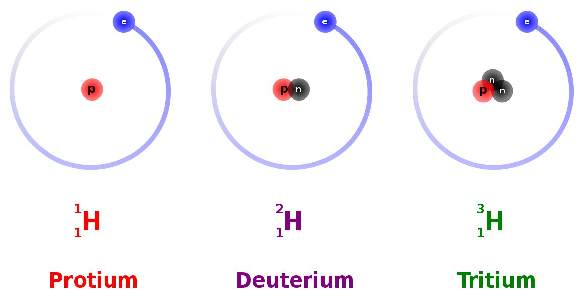
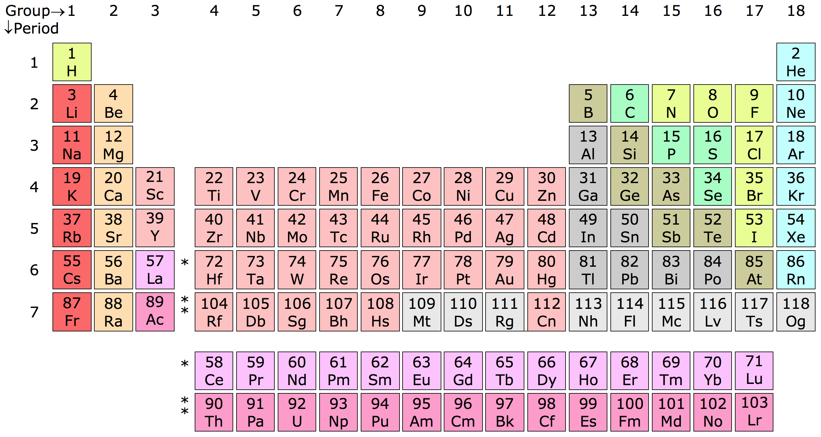
All elements on the Periodic Table of Elements (see chapter 3) contain isotopes. An isotope is an atom of an element with a different number of neutrons. For example, hydrogen (H) always has 1 proton in its nucleus (the atomic number), but the number of neutrons can vary among the isotopes (0, 1, 2). Recall that the number of neutrons added to the atomic number gives the atomic mass. When hydrogen has 1 proton and 0 neutrons it is sometimes called protium (1H), when hydrogen has 1 proton and 1 neutron it is called deuterium (2H), and when hydrogen has 1 proton and 2 neutrons it is called tritium (3H).
Many elements have both stable and unstable isotopes. For the hydrogen example, 1H and 2H are stable, but 3H is unstable. Unstable isotopes, called radioactive isotopes, spontaneously decay over time releasing subatomic particles or energy in a process called radioactive decay. When this occurs, an unstable isotope becomes a more stable isotope of another element. For example, carbon-14 (14C) decays to nitrogen-14 (14N).
The radioactive decay of any individual atom is a completely unpredictable and random event. However, some rock specimens have an enormous number of radioactive isotopes, perhaps trillions of atoms, and this large group of radioactive isotopes does have a predictable pattern of radioactive decay. The radioactive decay of half of the radioactive isotopes in this group takes a specific amount of time. The time it takes for half of the atoms in a substance to decay is called the half-life. In other words, the half-life of an isotope is the amount of time it takes for half of a group of unstable isotopes to decay to a stable isotope. The half-life is constant and measurable for a given radioactive isotope, so it can be used to calculate the age of a rock. For example, the half-life uranium-238 (238U) is 4.5 billion years and the half-life of 14C is 5,730 years.
The principles behind this dating method require two key assumptions. First, the mineral grains containing the isotope formed at the same time as the rock, such as minerals in an igneous rock that crystallized from magma. Second, the mineral crystals remain a closed system, meaning they are not subsequently altered by elements moving in or out of them.
These requirements place some constraints on the kinds of rock suitable for dating, with igneous rock being the best. Metamorphic rocks are crystalline, but the processes of metamorphism may reset the clock and derived ages may represent a smear of different metamorphic events rather than the age of original crystallization. Detrital sedimentary rocks contain clasts from separate parent rocks from unknown locations and derived ages are thus meaningless. However, sedimentary rocks with precipitated minerals, such as evaporites, may contain elements suitable for radioisotopic dating. Igneous pyroclastic layers and lava flows within a sedimentary sequence can be used to date the sequence. Cross-cutting igneous rocks and sills can be used to bracket the ages of affected, older sedimentary rocks. The resistant mineral zircon, found as clasts in many ancient sedimentary rocks, has been successfully used for establishing very old dates, including the age of Earth’s oldest known rocks. Knowing that zircon minerals in metamorphosed sediments came from older rocks that are no longer available for study, scientists can date zircon to establish the age of the pre-metamorphic source rocks.
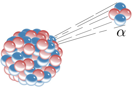
There are several ways radioactive atoms decay. We will consider three of them here—alpha decay, beta decay, and electron capture. Alpha decay is when an alpha particle, which consists of two protons and two neutrons, is emitted from the nucleus of an atom. This also happens to be the nucleus of a helium atom; helium gas may get trapped in the crystal lattice of a mineral in which alpha decay has taken place. When an atom loses two protons from its nucleus, lowering its atomic number, it is transformed into an element that is two atomic numbers lower on the Periodic Table of the Elements.
The loss of four particles, in this case two neutrons and two protons, also lowers the mass of the atom by four. For example alpha decay takes place in the unstable isotope 238U, which has an atomic number of 92 (92 protons) and mass number of 238 (total of all protons and neutrons). When 238U spontaneously emits an alpha particle, it becomes thorium-234 (234Th). The radioactive decay product of an element is called its daughter isotope and the original element is called the parent isotope. In this case, 238U is the parent isotope and 234Th is the daughter isotope. The half-life of 238U is 4.5 billion years, i.e., the time it takes for half of the parent isotope atoms to decay into the daughter isotope. This isotope of uranium, 238U, can be used for absolute dating the oldest materials found on Earth, and even meteorites and materials from the earliest events in our solar system.
Beta Decay
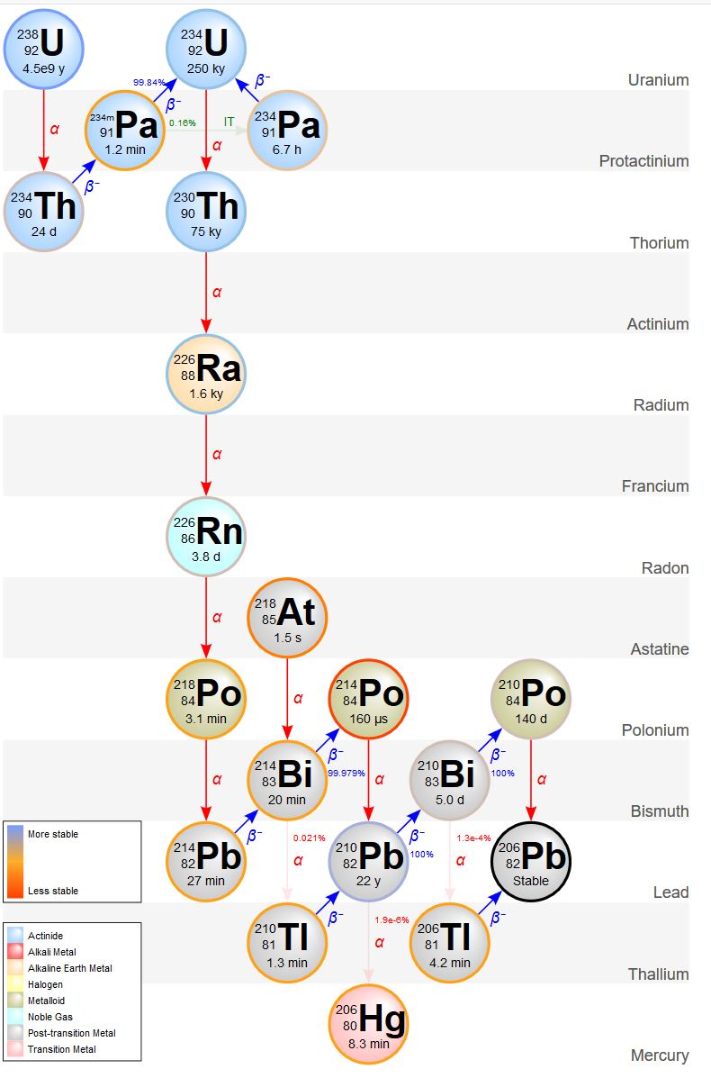
Beta decay is when a neutron in its nucleus splits into an electron and a proton. The electron is emitted from the nucleus as a beta ray. The new proton increases the element’s atomic number by one, forming a new element with the same atomic mass as the parent isotope. For example, 234Th is unstable and undergoes beta decay to form protactinium-234 (234Pa), which also undergoes beta decay to form uranium-234 (234U). Notice these are all isotopes of different elements but they have the same atomic mass of 234. The decay process of radioactive elements like uranium keeps producing radioactive parents and daughters until a stable, or non-radioactive, daughter is formed. Such a series is called a decay chain. The decay chain of the radioactive parent isotope 238U progresses through a series of alpha (red arrows on the adjacent figure) and beta decays (blue arrows), until it forms the stable daughter isotope, lead-206 (206Pb).
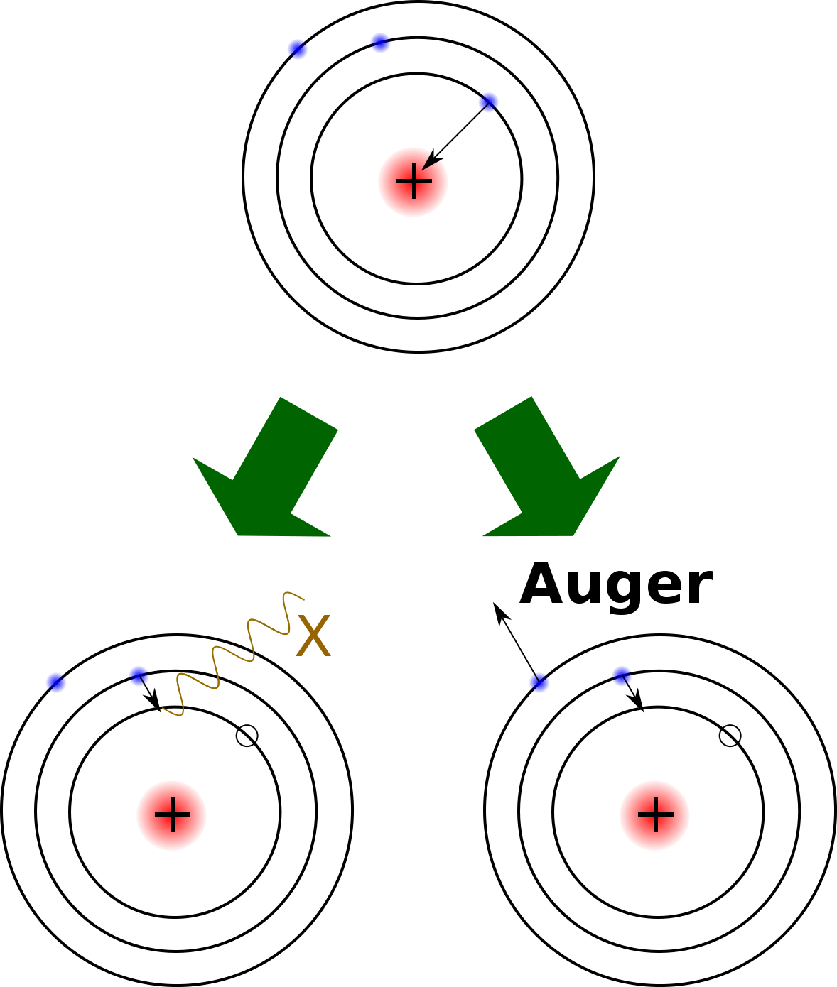
Electron capture is when a proton in the nucleus captures an electron from one of the electron shells and becomes a neutron. This produces one of two different effects: 1) an electron jumps in to fill the missing spot of the departed electron and emits an X-ray, or 2) in what is called the Auger process, another electron is released and changes the atom into an ion. The atomic number is reduced by one and mass number remains the same. An example of an element that decays by electron capture is potassium-40 (40K). Radioactive 40K makes up a tiny percentage (0.012%) of naturally occurring potassium, most of which not radioactive. 40K decays to argon-40 (40Ar) with a half-life of 1.25 billion years, so it is very useful for dating geological events. Below is a table of some of the more commonly-used radioactive dating isotopes and their half-lives.
| Elements | Parent symbol | Daughter symbol | Half-life |
|---|---|---|---|
| Uranium-238/Lead-206 | 238U | 206Pb | 4.5 billion years |
| Uranium-235/Lead-207 | 235U | 207Pb | 704 million years |
| Potassium-40/Argon-40 | 40K | 40Ar | 1.25 billion years |
| Rubidium-87/Strontium-87 | 87Rb | 87Sr | 48.8 billion years |
| Carbon-14/Nitrogen-14 | 14C | 14N | 5,730 years |
Table 7.1: Some common isotopes used for radioisotopic dating.
7.2.2 Radioisotopic Dating
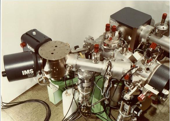
For a given a sample of rock, how is the dating procedure carried out? The parent and daughter isotopes are separated out of the mineral using chemical extraction. In the case of uranium, 238U and 235U isotopes are separated out together, as are the 206Pb and 207Pb with an instrument called a mass spectrometer.
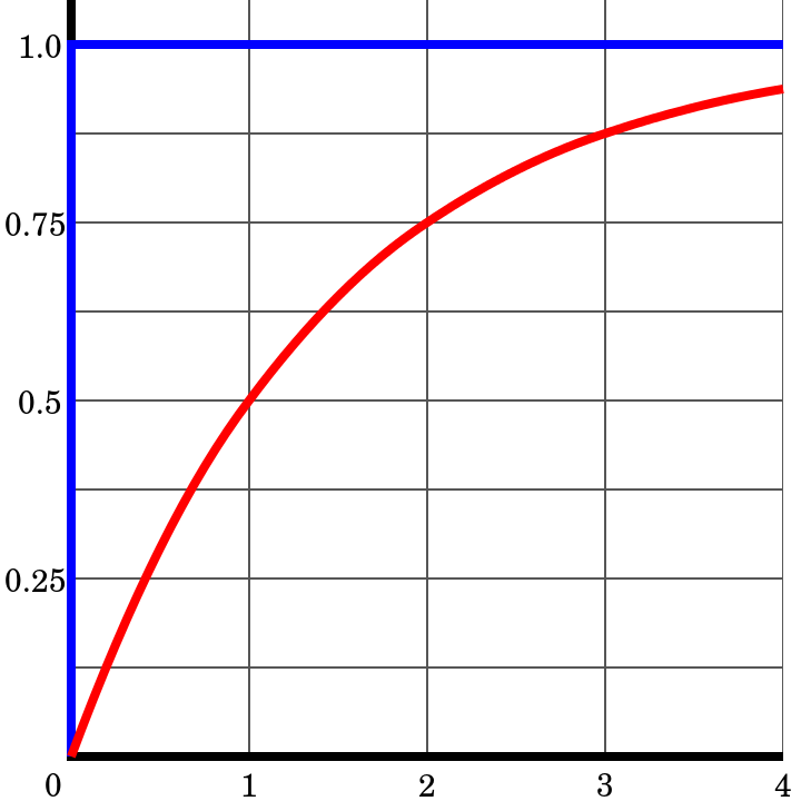
Here is a simple example of age calculation using the daughter-to-parent ratio of isotopes. When the mineral initially forms, it consists of 0% daughter and 100% parent isotope, so the daughter-to-parent ratio (D/P) is 0. After one half-life, half the parent has decayed so there is 50% daughter and 50% parent, a 50/50 ratio, with D/P = 1. After two half-lives, there is 75% daughter and 25% parent (75/25 ratio) and D/P = 3. This can be further calculated for a series of half-lives as shown in the table. The table does not show more than 10 half-lives because after about 10 half-lives, the amount of remaining parent is so small it becomes too difficult to accurately measure via chemical analysis. Modern applications of this method have achieved remarkable accuracies of plus or minus two million years in 2.5 billion years (that’s ±0.055%). Applying the uranium/lead technique in any given sample analysis provides two separate clocks running at the same time, 238U and 235U. The existence of these two clocks in the same sample gives a cross-check between the two. Many geological samples contain multiple parent/daughter pairs, so cross-checking the clocks confirms that radioisotopic dating is highly reliable.
| Half lives (#) | Parent present (%) | Daughter present (%) | Daughter/parent ratio | Parent/daughter ratio |
|---|---|---|---|---|
| Start the clock | 100 | 0 | 0 | Infinite |
| 1 | 50 | 50 | 1 | 1 |
| 2 | 25 | 75 | 3 | 0.33 |
| 3 | 12.5 | 87.5 | 7 | 0.143 |
| 4 | 6.25 | 93.75 | 15 | 0.0667 |
| 5 | 3.125 | 96.875 | 31 | 0.0325 |
| 10 | 0.098 | 99.9 | 1023 | 0.00098 |
Table 7.2: Ratio of parent to daughter in terms of half-life.

Another radioisotopic dating method involves carbon and is useful for dating archaeologically important samples containing organic substances like wood or bone. Radiocarbon dating, also called carbon dating, uses the unstable isotope carbon-14 (14C) and the stable isotope carbon-12 (12C). Carbon-14 is constantly being created in the atmosphere by the interaction of cosmic particles with atmospheric nitrogen-14 (14N). Cosmic particles such as neutrons strike the nitrogen nucleus, kicking out a proton but leaving the neutron in the nucleus. The collision reduces the atomic number by one, changing it from seven to six, changing the nitrogen into carbon with the same mass number of 14. The 14C quickly bonds with oxygen (O) in the atmosphere to form carbon dioxide (14CO2) that mixes with other atmospheric carbon dioxide (12CO2) and this mix of gases is incorporated into living matter. While an organism is alive, the ratio of 14C/12C in its body doesn’t really change since CO2 is constantly exchanged with the atmosphere. However, when it dies, the radiocarbon clock starts ticking as the 14C decays back to 14N by beta decay, which has a half-life of 5,730 years. The radiocarbon dating technique is thus useful for 57,300 years or so, about 10 half-lives back.
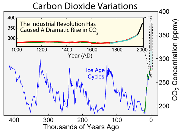
Radiocarbon dating relies on daughter-to-parent ratios derived from a known quantity of parent 14C. Early applications of carbon dating assumed the production and concentration of 14C in the atmosphere remained fairly constant for the last 50,000 years. However, it is now known that the amount of parent 14C levels in the atmosphere has varied. Comparisons of carbon ages with tree-ring data and other data for known events have allowed reliable calibration of the radiocarbon dating method. Taking into account carbon-14 baseline levels must be calibrated against other reliable dating methods, carbon dating has been shown to be a reliable method for dating archaeological specimens and very recent geologic events.
7.2.3 Age of the Earth
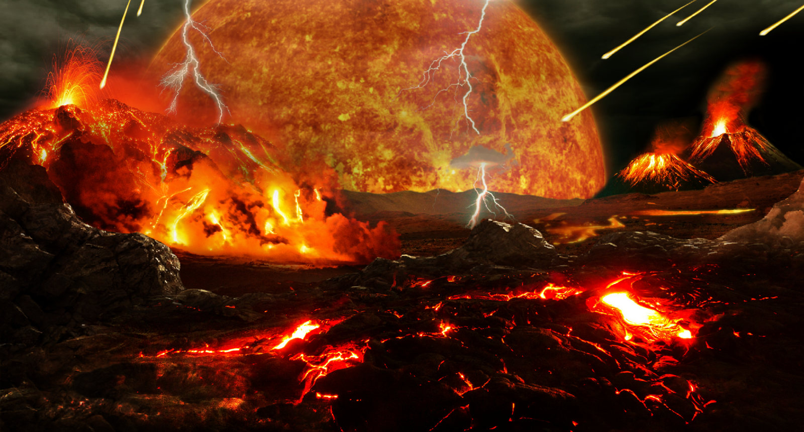
The work of Hutton and other scientists gained attention after the Renaissance (see chapter 1), spurring exploration into the idea of an ancient Earth. In the late 19th century William Thompson, a.k.a. Lord Kelvin, applied his knowledge of physics to develop the assumption that the Earth started as a hot molten sphere. He estimated the Earth is 98 million years old, but because of uncertainties in his calculations stated the age as a range of between 20 and 400 million years. This animation illustrates how Kelvin calculated this range and why his numbers were so far off, which has to do with unequal heat transfer within the Earth. It has also been pointed out that Kelvin failed to consider pliability and convection in the Earth’s mantle as a heat transfer mechanism. Kelvin’s estimate for Earth’s age was considered plausible but not without challenge, and the discovery of radioactivity provided a more accurate method for determining ancient ages.
In the 1950’s, Clair Patterson (1922–1995) thought he could determine the age of the Earth using radioactive isotopes from meteorites, which he considered to be early solar system remnants that were present at the time Earth was forming. Patterson analyzed meteorite samples for uranium and lead using a mass spectrometer. He used the uranium/lead dating technique in determining the age of the Earth to be 4.55 billion years, give or take about 70 million (± 1.5%). The current estimate for the age of the Earth is 4.54 billion years, give or take 50 million (± 1.1%). It is remarkable that Patterson, who was still a graduate student at the University of Chicago, came up with a result that has been little altered in over 60 years, even as technology has improved dating methods.
7.2.4 Dating Geological Events
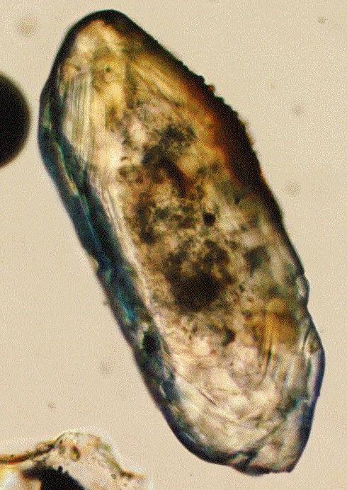
Radioactive isotopes of elements that are common in mineral crystals are useful for radioisotopic dating. The uranium/lead method, with its two cross-checking clocks, is most often used with crystals of the mineral zircon (ZrSiO4) where uranium can substitute for zirconium in the crystal lattice. Zircon is resistant to weathering which makes it useful for dating geological events in ancient rocks. During metamorphic events, zircon crystals may form multiple crystal layers, with each layer recording the isotopic age of an event, thus tracing the progress of the several metamorphic events.
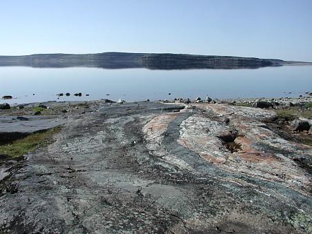
Geologists have used zircon grains to do some amazing studies that illustrate how scientific conclusions can change with technological advancements. Zircon crystals from Western Australia that formed when the crust first differentiated from the mantle 4.4 billion years ago have been determined to be the oldest known rocks. The zircon grains were incorporated into metasedimentary host rocks, sedimentary rocks showing signs of having undergone partial metamorphism. The host rocks were not very old but the embedded zircon grains were created 4.4 billion years ago, and survived the subsequent processes of weathering, erosion, deposition, and metamorphism. From other properties of the zircon crystals, researchers concluded that not only were continental rocks exposed above sea level, but also that conditions on the early Earth were cool enough for liquid water to exist on the surface. The presence of liquid water allowed the processes of weathering and erosion to take place. Researchers at UCLA studied 4.1 billion-year-old zircon crystals and found carbon in the zircon crystals that may be biogenic in origin, meaning that life may have existed on Earth much earlier than previously thought.
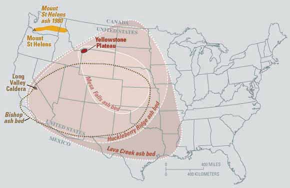
Igneous rocks best suited for radioisotopic dating because their primary minerals provide dates of crystallization from magma. Metamorphic processes tend to reset the clocks and smear the igneous rock’s original date. Detrital sedimentary rocks are less useful because they are made of minerals derived from multiple parent sources with potentially many dates. However, scientists can use igneous events to date sedimentary sequences. For example, if sedimentary strata are between a lava flow and volcanic ash bed with radioisotopic dates of 54 million years and 50 million years, then geologists know the sedimentary strata and its fossils formed between 54 and 50 million years ago. Another example would be a 65 million year old volcanic dike that cut across sedimentary strata. This provides an upper limit age on the sedimentary strata, so this strata would be older than 65 million years. Potassium is common in evaporite sediments and has been used for potassium/argon dating. Primary sedimentary minerals containing radioactive isotopes like 40K, has provided dates for important geologic events.
7.2.5 Other Absolute Dating Techniques
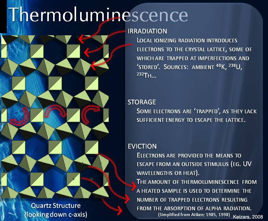
Luminescence (aka Thermoluminescence): Radioisotopic dating is not the only way scientists determine numeric ages. Luminescence dating measures the time elapsed since some silicate minerals, such as coarse-sediments of silicate minerals, were last exposed to light or heat at the surface of Earth. All buried sediments are exposed to radiation from normal background radiation from the decay process described above. Some of these electrons get trapped in the crystal lattice of silicate minerals like quartz. When exposed at the surface, ultraviolet radiation and heat from the Sun releases these electrons, but when the minerals are buried just a few inches below the surface, the electrons get trapped again. Samples of coarse sediments collected just a few feet below the surface are analyzed by stimulating them with light in a lab. This stimulation releases the trapped electrons as a photon of light which is called luminescence. The amount luminescence released indicates how long the sediment has been buried. Luminescence dating is only useful for dating young sediments that are less than 1 million years old. In Utah, luminescence dating is used to determine when coarse-grained sediment layers were buried near a fault. This is one technique used to determine the recurrence interval of large earthquakes on faults like the Wasatch Fault that primarily cut coarse-grained material and lack buried organic soils for radiocarbon dating.
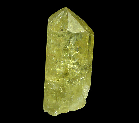
Fission Track: Fission track dating relies on damage to the crystal lattice produced when unstable 238U decays to the daughter product 234Th and releases an alpha particle. These two decay products move in opposite directions from each other through the crystal lattice leaving a visible track of damage. This is common in uranium-bearing mineral grains such as apatite. The tracks are large and can be visually counted under an optical microscope. The number of tracks correspond to the age of the grains. Fission track dating works from about 100,000 to 2 billion (1 × 10⁵ to 2 × 10⁹) years ago. Fission track dating has also been used as a second clock to confirm dates obtained by other methods.

Take this quiz to check your comprehension of this section.
If you are using an offline version of this text, access the quiz for section 7.2 via the QR code.
7.3 Fossils and Evolution
Fossils are any evidence of past life preserved in rocks. They may be actual remains of body parts (rare), impressions of soft body parts, casts and molds of body parts (more common), body parts replaced by mineral (common) or evidence of animal behavior such as footprints and burrows. The body parts of living organisms range from the hard bones and shells of animals, soft cellulose of plants, soft bodies of jellyfish, down to single cells of bacteria and algae. Which body parts can be preserved? The vast majority of life today consists soft-bodied and/or single celled organisms, and will not likely be preserved in the geologic record except under unusual conditions. The best environment for preservation is the ocean, yet marine processes can dissolve hard parts and scavenging can reduce or eliminate remains. Thus, even under ideal conditions in the ocean, the likelihood of preservation is quite limited. For terrestrial life, the possibility of remains being buried and preserved is even more limited. In other words, the fossil record is incomplete and records only a small percentage of life that existed. Although incomplete, fossil records are used for stratigraphic correlation, using the Principle of Faunal Succession, and provide a method used for establishing the age of a formation on the Geologic Time Scale.
7.3.1 Types of Preservation
Remnants or impressions of hard parts, such as a marine clam shell or dinosaur bone, are the most common types of fossils. The original material has almost always been replaced with new minerals that preserve much of the shape of the original shell, bone, or cell. The common types of fossil preservation are actual preservation, permineralization, molds and casts, carbonization, and trace fossils.
Actual preservation is a rare form of fossilization where the original materials or hard parts of the organism are preserved. Preservation of soft-tissue is very rare since these organic materials easily disappear because of bacterial decay. Examples of actual preservation are unaltered biological materials like insects in amber or original minerals like mother-of-pearl on the interior of a shell. Another example is mammoth skin and hair preserved in post-glacial deposits in the Arctic regions. Rare mummification has left fragments of soft tissue, skin, and sometimes even blood vessels of dinosaurs, from which proteins have been isolated and evidence for DNA fragments have been discovered.

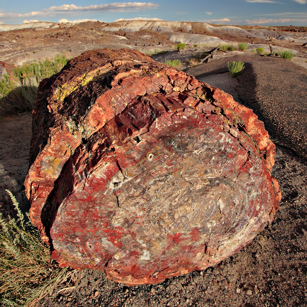
Permineralization occurs when an organism is buried, and then elements in groundwater completely impregnate all spaces within the body, even cells. Soft body structures can be preserved in great detail, but stronger materials like bone and teeth are the most likely to be preserved. Petrified wood is an example of detailed cellulose structures in the wood being preserved. The University of California Berkeley website has more information on permineralization.
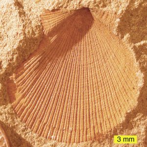
Molds and casts form when the original material of the organism dissolves and leaves a cavity in the surrounding rock. The shape of this cavity is an external mold. If the mold is subsequently filled with sediments or a mineral precipitate, the organism’s external shape is preserved as a cast. Sometimes internal cavities of organisms, such internal casts of clams, snails, and even skulls are preserved as internal casts showing details of soft structures. If the chemistry is right, and burial is rapid, mineral nodules form around soft structures preserving the three-dimensional detail. This is called authigenic mineralization.
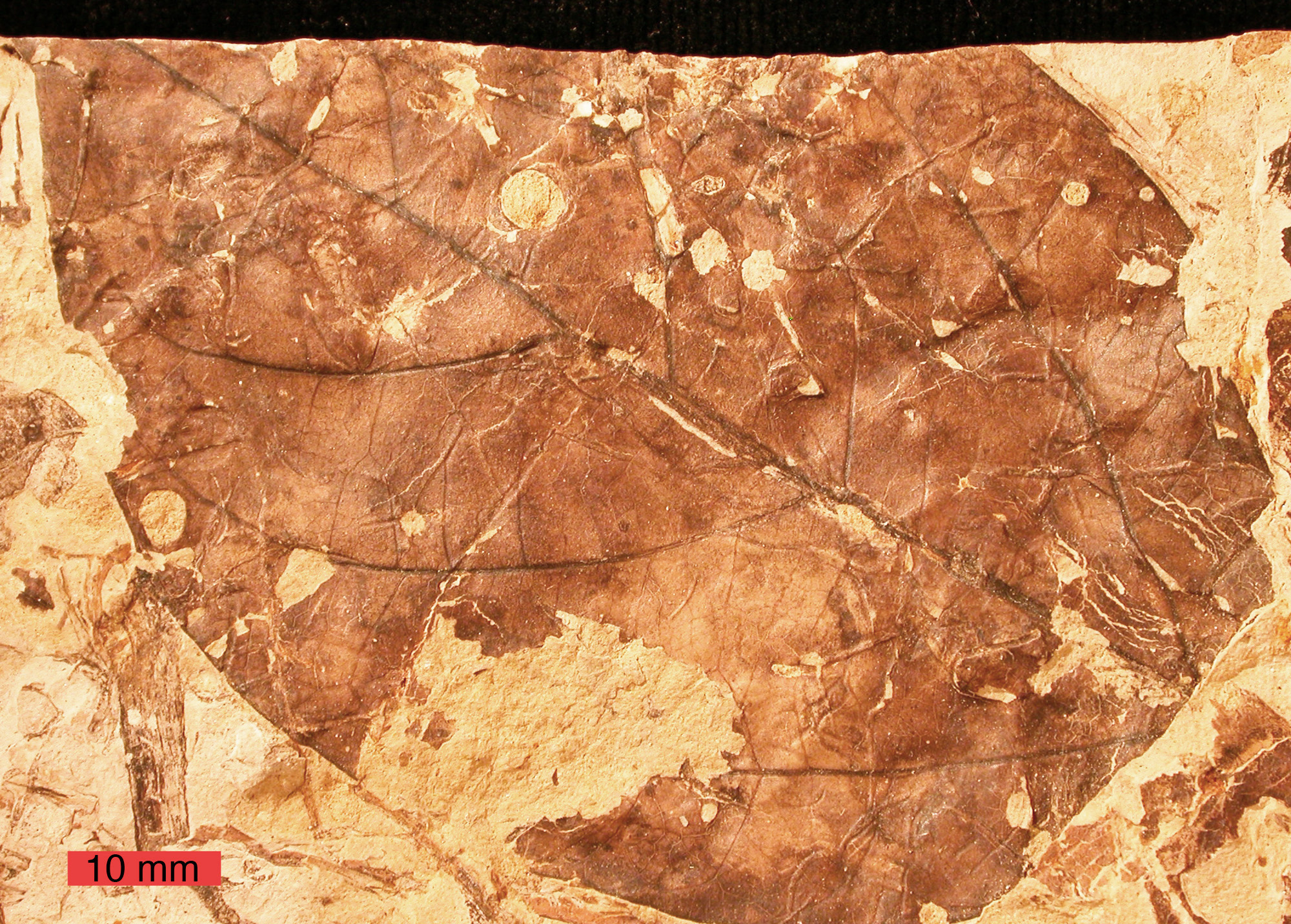
Carbonization occurs when the organic tissues of an organism are compressed, the volatiles are driven out, and everything but the carbon disappears leaving a carbon silhouette of the original organism. Leaf and fern fossils are examples of carbonization.

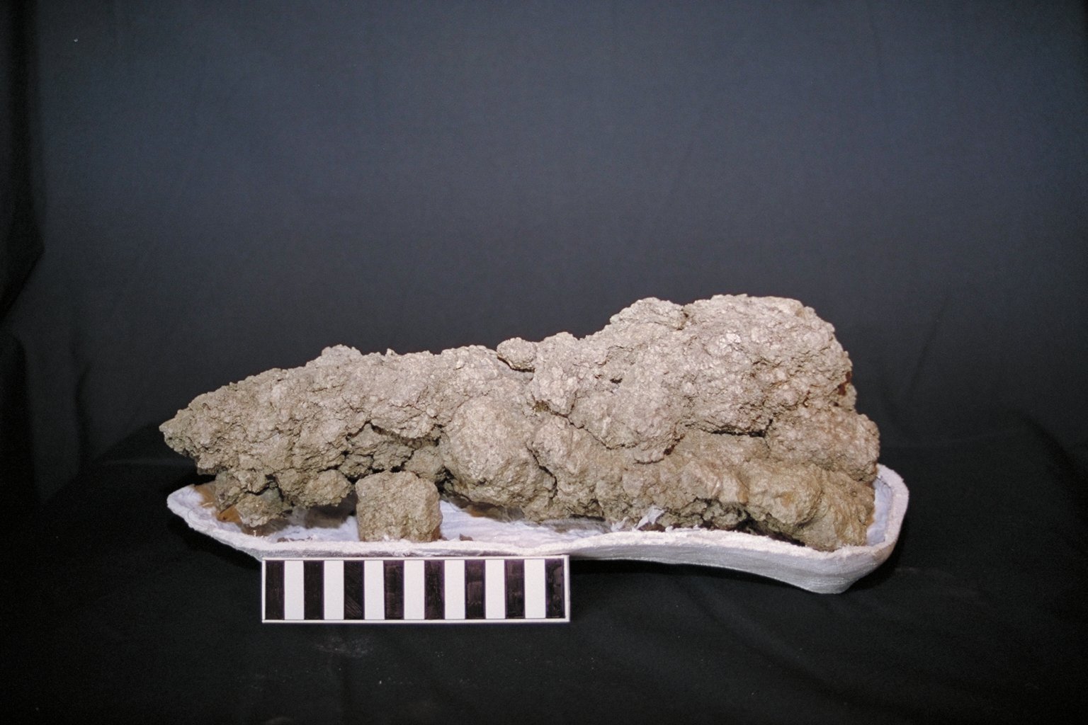
Trace fossils are indirect evidence left behind by an organism, such as burrows and footprints, as it lived its life. Ichnology is specifically the study of prehistoric animal tracks. Dinosaur tracks testify to their presence and movement over an area, and even provide information about their size, gait, speed, and behavior. Burrows dug by tunneling organisms tell of their presence and mode of life. Other trace fossils include fossilized feces called coprolites and stomach stones called gastroliths that provide information about diet and habitat.
7.3.2 Evolution
Evolution has created a variety of ancient fossils that are important to stratigraphic correlation. (see chapter 7 and chapter 5) This section is a brief discussion of the process of evolution. The British naturalist Charles Darwin (1809-1882) recognized that life forms evolve into progeny life forms. He proposed natural selection—which operated on organisms living under environmental conditions that posed challenges to survival—was the mechanism driving the process of evolution forward.
The basic classification unit of life is the species: a population of organisms that exhibit shared characteristics and are capable of reproducing fertile offspring. For a species to survive, each individual within a particular population is faced with challenges posed by the environment and must survive them long enough to reproduce. Within the natural variations present in the population, there may be individuals possessing characteristics that give them some advantage in facing the environmental challenges. These individuals are more likely to reproduce and pass these favored characteristics on to successive generations. If sufficient individuals in a population fail to surmount the challenges of the environment and the population cannot produce enough viable offspring, the species becomes extinct. The average lifespan of a species in the fossil record is around a million years. That life still exists on Earth shows the role and importance of evolution as a natural process in meeting the continual challenges posed by our dynamic Earth. If the inheritance of certain distinctive characteristics is sufficiently favored over time, populations may become genetically isolated from one another, eventually resulting in the evolution of separate species. This genetic isolation may also be caused by a geographic barrier, such as an island surrounded by ocean. This theory of evolution by natural selection was elaborated by Darwin in his book On the Origin of Species (see chapter 1). Since Darwin’s original ideas, technology has provided many tools and mechanisms to study how evolution and speciation take place and this arsenal of tools is growing. Evolution is well beyond the hypothesis stage and is a well-established theory of modern science.
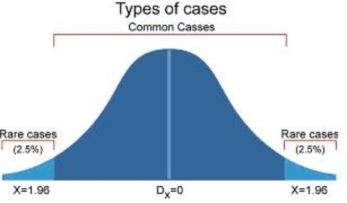
Variation within populations occurs by the natural mixing of genes through sexual reproduction or from naturally occurring mutations. Some of this genetic variation can introduce advantageous characteristics that increase the individual’s chances of survival. While some species in the fossil record show little morphological change over time, others show gradual or punctuated changes, within which intermediate forms can be seen.

Take this quiz to check your comprehension of this section.
If you are using an offline version of this text, access the quiz for section 7.3 via the QR code.
7.4 Correlation
Correlation is the process of establishing which sedimentary strata are of the same age but geographically separate. Correlation can be determined by using magnetic polarity reversals (chapter 2), rock types, unique rock sequences, or index fossils. There are four main types of correlation: stratigraphic, lithostratigraphic, chronostratigraphic, and biostratigraphic.
7.4.1 Stratigraphic Correlation
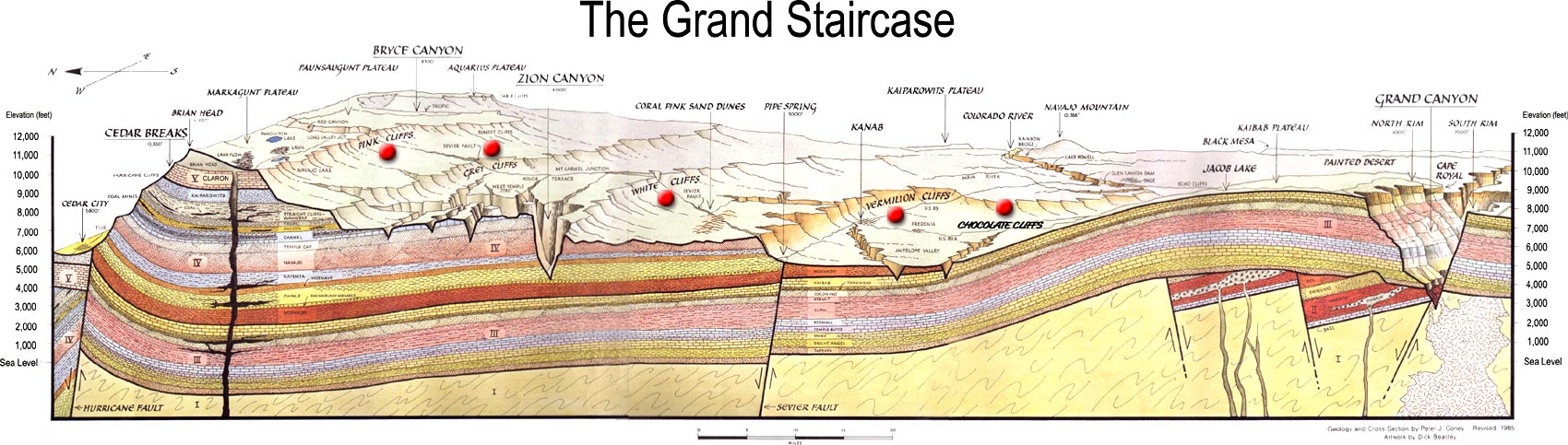
Stratigraphic correlation is the process of establishing which sedimentary strata are the same age at distant geographical areas by means of their stratigraphic relationship. Geologists construct geologic histories of areas by mapping and making stratigraphic columns-a detailed description of the strata from bottom to top. An example of stratigraphic relationships and correlation between Canyonlands National Park and Zion National Park in Utah. At Canyonlands, the Navajo Sandstone overlies the Kayenta Formation which overlies the cliff-forming Wingate Formation. In Zion, the Navajo Sandstone overlies the Kayenta Formation which overlies the cliff-forming Moenave Formation. Based on the stratigraphic relationship, the Wingate and Moenave Formations correlate. These two formations have unique names because their composition and outcrop pattern is slightly different. Other strata in the Colorado Plateau and their sequence can be recognized and correlated over thousands of square miles.
7.4.2 Lithostratigraphic Correlation

Lithostratigraphic correlation establishes a similar age of strata based on the lithology that is the composition and physical properties of that strata. Lithos is Greek for stone and -logy comes from the Greek word for doctrine or science. Lithostratigraphic correlation can be used to correlate whole formations long distances or can be used to correlate smaller strata within formations to trace their extent and regional depositional environments.
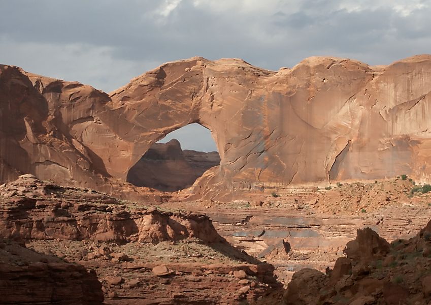
For example, the Navajo Sandstone, which makes up the prominent walls of Zion National Park, is the same Navajo Sandstone in Canyonlands because the lithology of the two are identical even though they are hundreds of miles apart. Extensions of the same Navajo Sandstone formation are found miles away in other parts of southern Utah, including Capitol Reef and Arches National Parks. Further, this same formation is the called the Aztec Sandstone in Nevada and Nugget Sandstone near Salt Lake City because they are lithologically distinct enough to warrant new names.
7.4.3 Chronostratigraphic Correlation
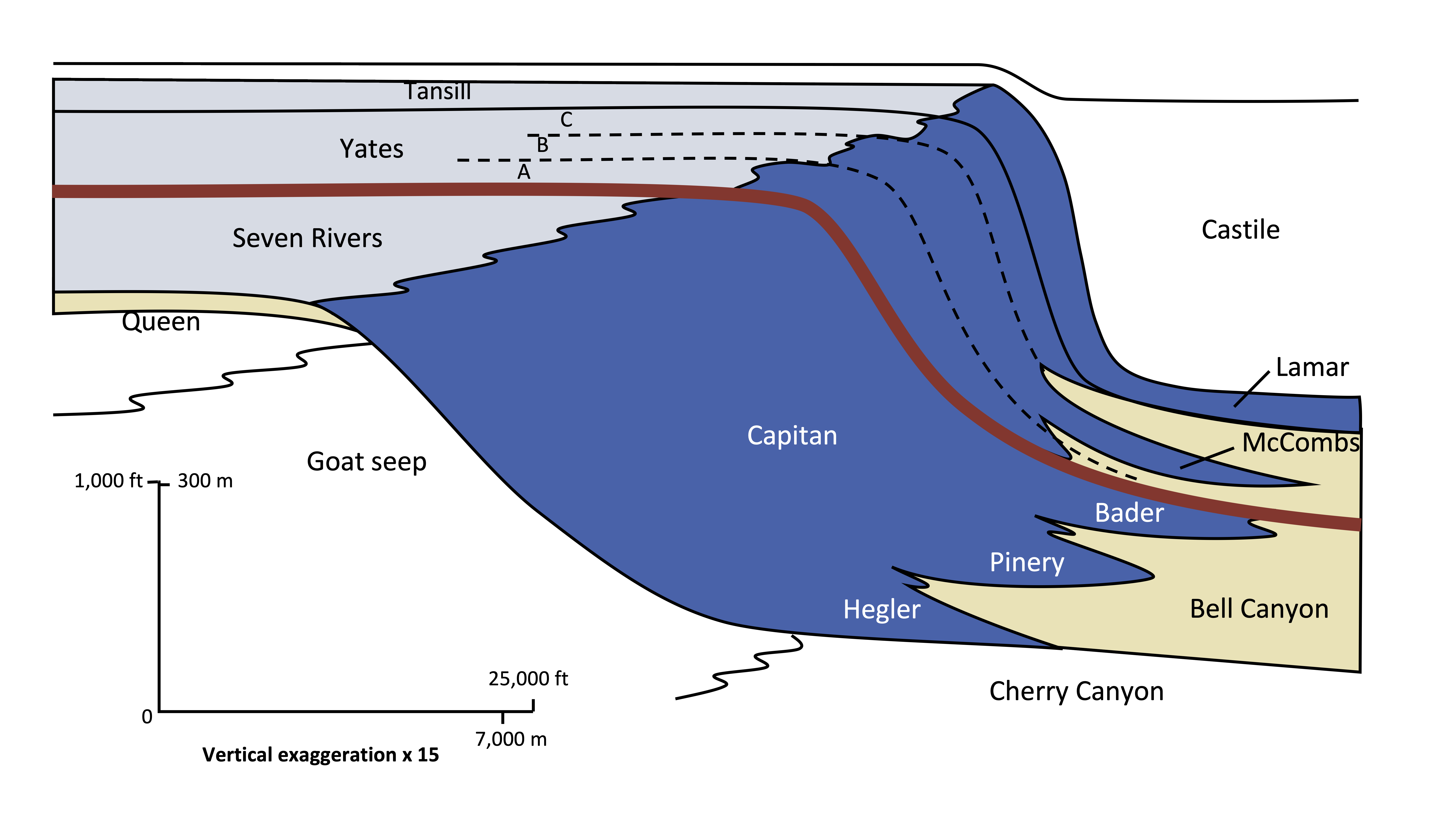
Chronostratigraphic correlation matches rocks of the same age, even though they are made of different lithologies. Different lithologies of sedimentary rocks can form at the same time at different geographic locations because depositional environments vary geographically. For example, at any one time in a marine setting there could be this sequence of depositional environments from beach to deep marine: beach, near shore area, shallow marine lagoon, reef, slope, and deep marine. Each depositional environment will have a unique sedimentary rock formation. On the figure of the Permian Capitan Reef at Guadalupe National Monument in West Texas, the red line shows a chronostratigraphic time line that represents a snapshot in time. Shallow-water marine lagoon/back reef area is light blue, the main Capitan reef is dark blue, and deep-water marine siltstone is yellow. All three of these unique lithologies were forming at the same time in Permian along this red timeline.
7.4.4 Biostratigraphic Correlation
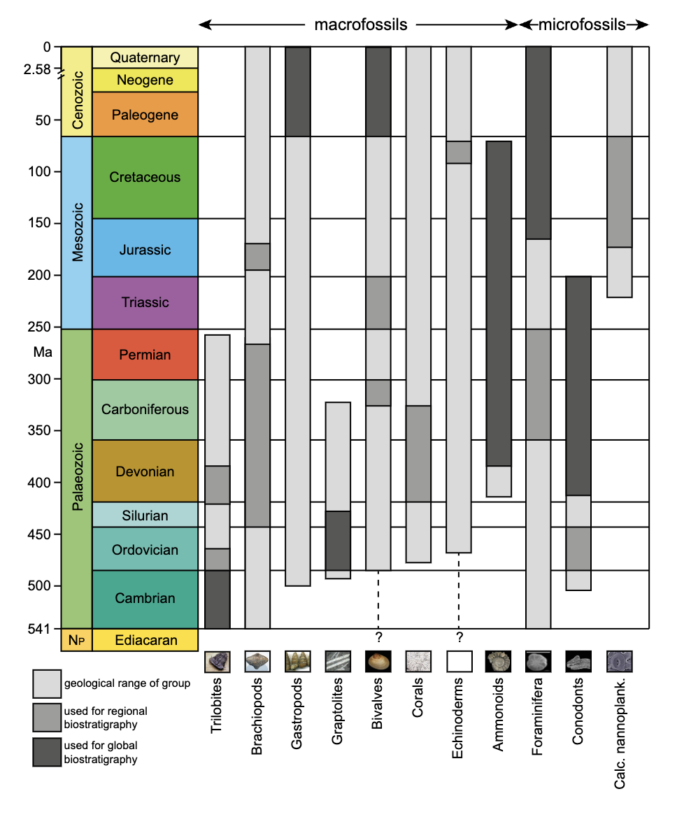
Biostratigraphic correlation uses index fossils to determine strata ages. Index fossils represent assemblages or groups of organisms that were uniquely present during specific intervals of geologic time. Assemblages is referring a group of fossils. Fossils allow geologists to assign a formation to an absolute date range, such as the Jurassic Period (199 to 145 million years ago), rather than a relative time scale. In fact, most of the geologic time ranges are mapped to fossil assemblages. The most useful index fossils come from lifeforms that were geographically widespread and had a species lifespan that was limited to a narrow time interval. In other words, index fossils can be found in many places around the world, but only during a narrow time frame. Some of the best fossils for biostratigraphic correlation are microfossils, most of which came from single-celled organisms.
As with microscopic organisms today, they were widely distributed across many environments throughout the world. Some of these microscopic organisms had hard parts, such as exoskeletons or outer shells, making them better candidates for preservation.
Foraminifera, single celled organisms with calcareous shells, are an example of an especially useful index fossil for the Cretaceous Period and Cenozoic Era.
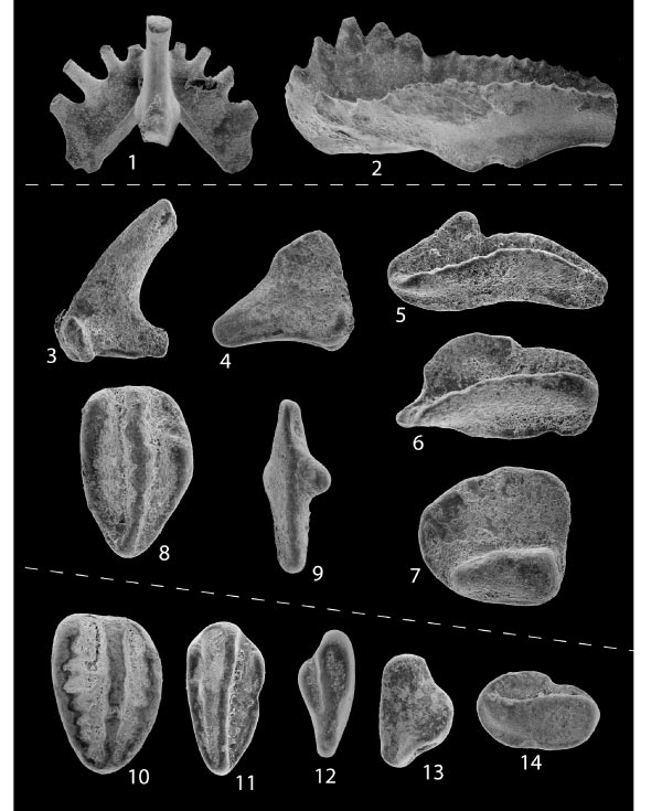
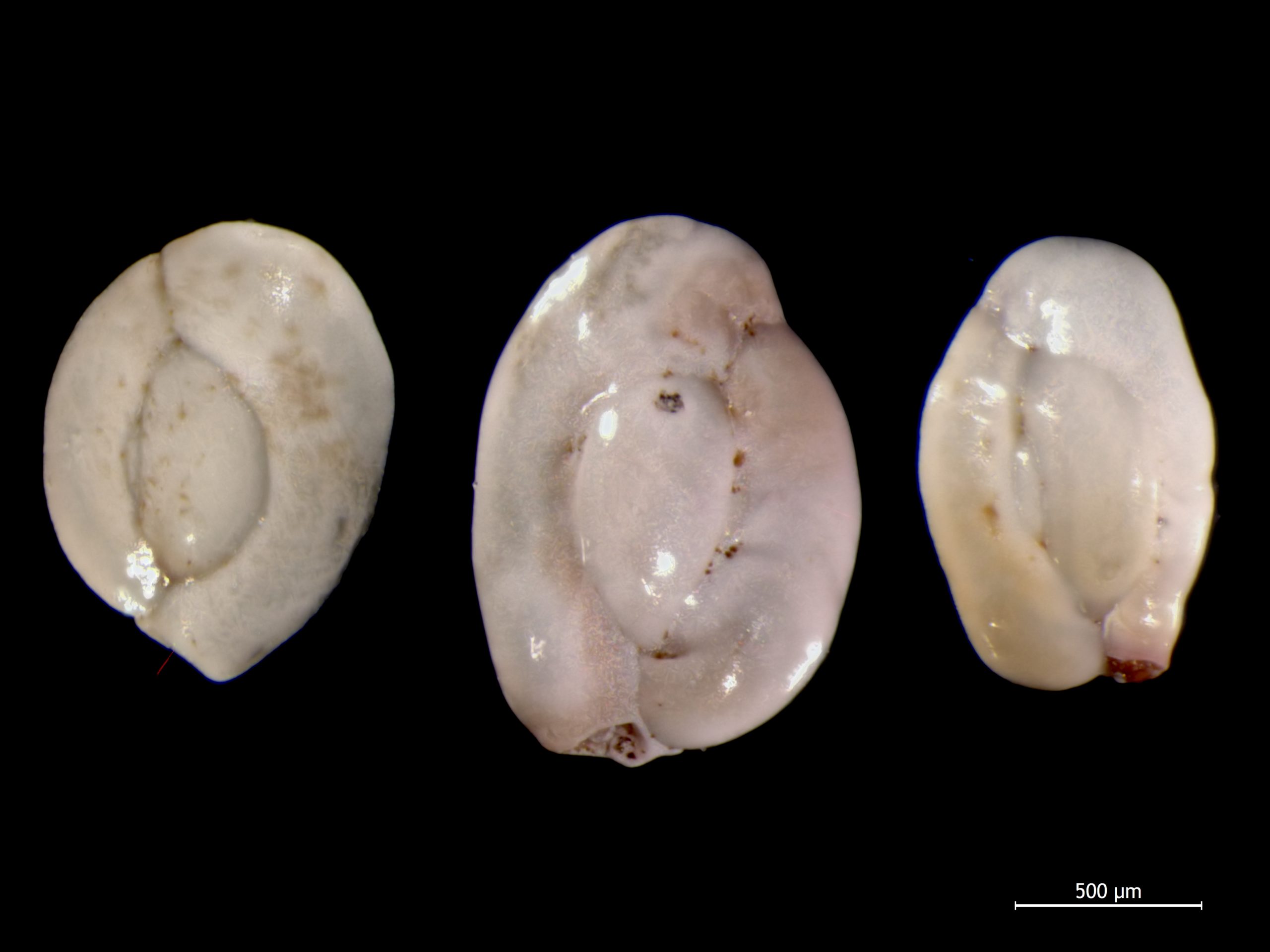
Conodonts are another example of microfossils useful for biostratigraphic correlation of the Cambrian through Triassic Periods. Conodonts are tooth-like phosphatic structures of an eel-like multi-celled organism that had no other preservable hard parts. The conodont-bearing creatures lived in shallow marine environments all over the world. Upon death, the phosphatic hard parts were scattered into the rest of the marine sediments. These distinctive tooth-like structures are easily collected and separated from limestone in the laboratory.
Because the conodont creatures were so widely abundant, rapidly evolving, and readily preserved in sediments, their fossils are especially useful for correlating strata, even though knowledge of the actual animal possessing them is sparse. Scientists in the 1960s carried out a fundamental biostratigraphic correlation that tied Triassic conodont zonation into ammonoids, which are extinct ancient cousins of the pearly nautilus. Up to that point ammonoids were the only standard for Triassic correlation, so cross-referencing micro- and macro-index fossils enhanced the reliability of biostratigraphic correlation for either type. That conodont study went on to establish the use of conodonts to internationally correlate Triassic strata located in Europe, Western North America, and the Arctic Islands of Canada.
7.4.5 Geologic Time Scale
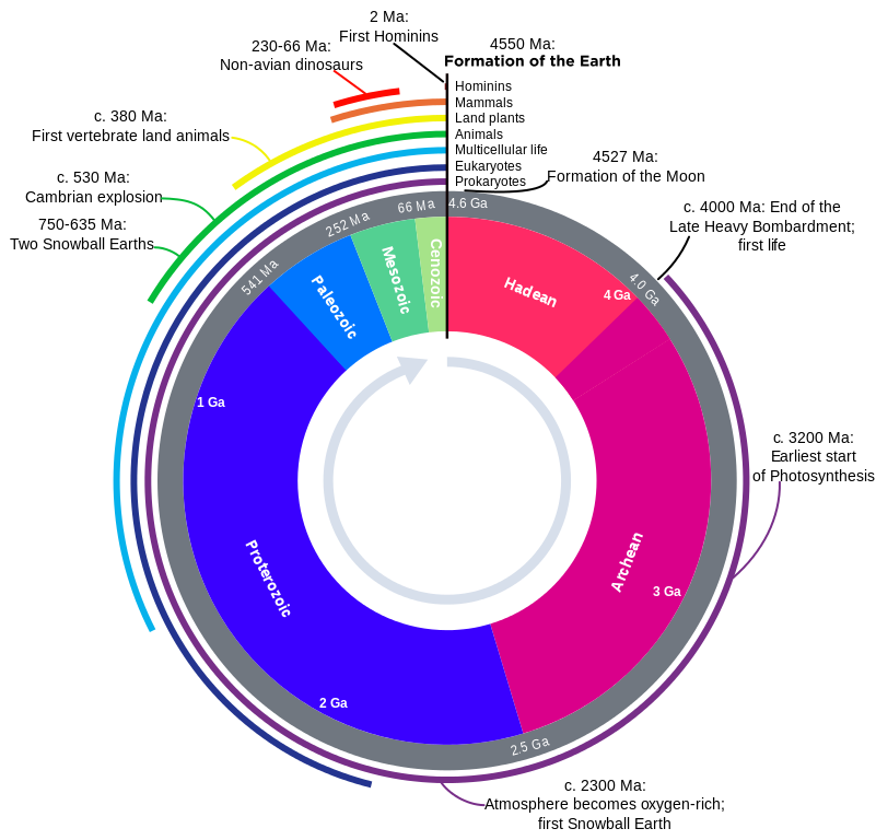
Geologic time has been subdivided into a series of divisions by geologists. Eon is the largest division of time, followed by era, period, epoch, and age. The partitions of the geologic time scale is the same everywhere on Earth; however, rocks may or may not be present at a given location depending on the geologic activity going on during a particular period of time. Thus, we have the concept of time vs. rock, in which time is an unbroken continuum but rocks may be missing and/or unavailable for study. The figure of the geologic time scale, represents time flowing continuously from the beginning of the Earth, with the time units presented in an unbroken sequence. But that does not mean there are rocks available for study for all of these time units.
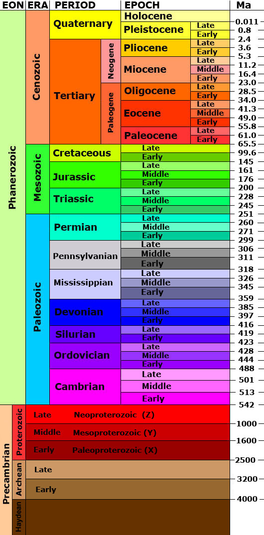
The geologic time scale was developed during the 19th century using the principles of stratigraphy. The relative order of the time units was determined before geologist had the tools to assign numerical ages to periods and events. Biostratigraphic correlation using fossils to assign era and period names to sedimentary rocks on a worldwide scale. With the expansion of science and technology, some geologists think the influence of humanity on natural processes has become so great they are suggesting a new geologic time period, known as the Anthropocene.

Take this quiz to check your comprehension of this section.
If you are using an offline version of this text, access the quiz for section 7.4 via the QR code.
Summary
Events in Earth history can be placed in sequence using the five principles of relative dating. The geologic time scale was completely worked out in the 19th Century using these principles without knowing any actual numeric ages for the events. The discovery of radioactivity in the late 1800s enabled absolute dating, the assignment of numerical ages to events in the Earth’s history, using decay of unstable radioactive isotopes. Accurately interpreting radioisotopic dating data depends on the type of rock tested and accurate assumptions about isotope baseline values. With a combination of relative and absolute dating, the history of geological events, age of Earth, and a geologic time scale have been determined with considerable accuracy. Stratigraphic correlation is additional tool used for understanding how depositional environments change geographically. Geologic time is vast, providing plenty of time for the evolution of various lifeforms, and some of these have become preserved as fossils that can be used for biostratigraphic correlation. The geologic time scale is continuous, although the rock record may be broken because rocks representing certain time periods may be missing.

Take this quiz to check your comprehension of this chapter.
If you are using an offline version of this text, access the quiz for chapter 7 via the QR code.
URLs Linked Within This Chapter
Animation 1: Why is it Hot Underground? [Video: 1:49] https://www.youtube.com/watch?v=mOSpRzW2i_4
The University of California Berkeley website: https://ucmp.berkeley.edu/paleo/fossils/permin.html
Text References
- Allison, P.A., and Briggs, D.E.G., 1993, Exceptional fossil record: Distribution of soft-tissue preservation through the Phanerozoic: Geology, v. 21, no. 6, p. 527–530.
- Bell, E.A., Boehnke, P., Harrison, T.M., and Mao, W.L., 2015, Potentially biogenic carbon preserved in a 4.1 billion-year-old zircon: Proc. Natl. Acad. Sci. U. S. A., v. 112, no. 47, p. 14518–14521.
- Brent Dalrymple, G., 1994, The Age of the Earth: Stanford University Press.
- Burleigh, R., 1981, W. F. Libby and the development of radiocarbon dating: Antiquity, v. 55, no. 214, p. 96–98.
- Christopher B. DuRoss, Stephen F. Personius, Anthony J. Crone, Susan S. Olig, and William R. Lund, 2011, Integration of Paleoseismic Data from Multiple Sites to Develop an Objective Earthquake Chronology: Application to the Weber Segment of the Wasatch Fault Zone, Utah: Bulletin of the Seismological Society of America, v. 101, no. 6, p. 2765–2781., doi: 0.1785/0120110102.
- Dass, C., 2007, Basics of mass spectrometry, in Fundamentals of Contemporary Mass Spectrometry: John Wiley & Sons, Inc., p. 1–14.
- Elston, D.P., Billingsley, G.H., and Young, R.A., 1989, Geology of Grand Canyon, Northern Arizona (with Colorado River Guides): Lees Ferry to Pierce Ferry, Arizona: Amer Geophysical Union.
- Erickson, J., Coates, D.R., and Erickson, H.P., 2014, An introduction to fossils and minerals: seeking clues to the Earth’s past: Facts on File science library, Facts On File, Incorporated, Facts on File science library.
- Geyh, M.A., and Schleicher, H., 1990, Absolute Age Determination: Physical and Chemical Dating Methods and Their Application, 503 pp: Spring-er-Verlag, New York.
- Ireland, T., 1999, New tools for isotopic analysis: Science, v. 286, no. 5448, p. 2289–2290.
- Jackson, P.W., and of London, G.S., 2007, Four Centuries of Geological Travel: The Search for Knowledge on Foot, Bicycle, Sledge and Camel: Geological Society special publication, Geological Society, Geological Society special publication.
- Jaffey, A.H., Flynn, K.F., Glendenin, L.E., Bentley, W.C., and others, 1971, Precision measurement of half-lives and specific activities of U 235 and U 238: Phys. Rev. C Nucl. Phys.
- Léost, I., Féraud, G., Blanc-Valleron, M.M., and Rouchy, J.M., 2001, First absolute dating of Miocene Langbeinite evaporites by 40Ar/39Ar laser step-heating:[K2Mg2 (SO4) 3] Stebnyk Mine (Carpathian Foredeep Basin): Geophys. Res. Lett., v. 28, no. 23, p. 4347–4350.
- Mosher, L.C., 1968, Triassic conodonts from Western North America and Europe and Their Correlation: J. Paleontol., v. 42, no. 4, p. 895–946.
- Oberthür, T., Davis, D.W., Blenkinsop, T.G., and Höhndorf, A., 2002, Precise U–Pb mineral ages, Rb–Sr and Sm–Nd systematics for the Great Dyke, Zimbabwe—constraints on late Archean events in the Zimbabwe craton and Limpopo belt: Precambrian Res., v. 113, no. 3–4, p. 293–305.
- Patterson, C., 1956, Age of meteorites and the earth: Geochim. Cosmochim. Acta, v. 10, no. 4, p. 230–237.
- Schweitzer, M.H., Wittmeyer, J.L., Horner, J.R., and Toporski, J.K., 2005, Soft-tissue vessels and cellular preservation in Tyrannosaurus rex: Science, v. 307, no. 5717, p. 1952–1955.
- Valley, J.W., Peck, W.H., King, E.M., and Wilde, S.A., 2002, A cool early Earth: Geology, v. 30, no. 4, p. 351–354.
- Whewell, W., 1837, History of the Inductive Sciences: From the Earliest to the Present Times: J.W. Parker, 492 p.
- Wilde, S.A., Valley, J.W., Peck, W.H., and Graham, C.M., 2001, Evidence from detrital zircons for the existence of continental crust and oceans on the Earth 4.4 Gyr ago: Nature, v. 409, no. 6817, p. 175–178.
- Winchester, S., 2009, The Map That Changed the World: William Smith and the Birth of Modern Geology: HarperCollins.
Figure References
Figure 7.1: Nicolas Steno, c. 1670. Justus Sustermans. ca. 1666 and 1677; uploaded in 2012. Public domain. https://commons.wikimedia.org/wiki/File:Portrait_of_Nicolas_Stenonus.jpg
Figure 7.2: Geologic time scale. USGS. 1997. Public domain. https://pubs.usgs.gov/gip/fossils/numeric.html
Figure 7.3: Lower strata are older than those lying on top of them. Wilson44691. 2009. Public domain. https://commons.wikimedia.org/wiki/File:IsfjordenSuperposition.jpg
Figure 7.4: Lateral continuity. Roger Bolsius. 2013. CC BY-SA 3.0. https://en.wikipedia.org/wiki/File:Grand_Canyon_Panorama_2013.jpg
Figure 7.5: Dark dike cutting across older rocks, the lighter of which is younger than the grey rock. Thomas Eliasson of Geological Survey of Sweden. 2008. CC BY 2.0. https://commons.wikimedia.org/wiki/File:Multiple_Igneous_Intrusion_Phases_Kosterhavet_Sweden.jpg
Figure 7.6: Fossil succession showing correlation among strata. דקי 2010. CC BY-SA 3.0. https://commons.wikimedia.org/wiki/File:Faunal_sucession.jpg
Figure 7.7: The Grand Canyon of Arizona. Jean-Christophe BENOIST. 2012. CC BY 3.0. https://commons.wikimedia.org/wiki/File:Grand_Canyon_-_Hopi_Point.JPG
Figure 7.8: The rocks of the Grand Canyon. NPS. 2018. Public domain. https://www.nps.gov/articles/age-of-rocks-in-grand-canyon.htm
Figure 7.9: The red, layered rocks of the Grand Canyon Supergroup overlying the dark-colored rocks of the Vishnu schist represents a type of unconformity called a nonconformity. Simeon87. 2012. CC BY-SA 3.0. https://commons.wikimedia.org/wiki/File:Grand_Canyon_with_Snow_4.JPG
Figure 7.10: All three of these formations have a disconformity at the two contacts between them. NPS. 2009. Public domain. https://commons.wikimedia.org/wiki/File:Redwall,_Temple_Butte_and_Muav_formations_in_Grand_Canyon.jpg
Figure 7.11: In the lower part of the picture is an angular unconformity in the Grand Canyon known as the Great Unconformity. Doug Dolde. 2008. Public domain. https://commons.wikimedia.org/wiki/File:View_from_Lipan_Point.jpg
Figure 7.12: Disconformity. דקי. 2008. CC BY-SA 3.0. https://commons.wikimedia.org/wiki/File:Disconformity.jpg
Figure 7.13: Nonconformity (the lower rocks are igneous or metamorphic). דקי. 2008. CC BY-SA 3.0. https://commons.wikimedia.org/wiki/File:Nonconformity.jpg
Figure 7.14: Angular unconformity. דקי. 2008. CC BY-SA 3.0. https://commons.wikimedia.org/wiki/File:Angular_unconformity.jpg
Figure 7.15: Block diagram to apply relative dating principles. Woudloper. 2009. CC BY-SA 1.0. https://commons.wikimedia.org/wiki/File:Cross-cutting_relations.svg
Figure 7.16: Canada’s Nuvvuagittuq Greenstone Belt may have the oldest rocks and oldest evidence life on Earth, according to recent studies. NASA. 2008. Public domain. https://commons.wikimedia.org/wiki/File:Nuvvuagittuq_belt_rocks.jpg
Figure 7.17: Three isotopes of hydrogen. Dirk Hünniger. 2016. CC BY-SA 3.0. https://commons.wikimedia.org/wiki/File:Hydrogen_Deuterium_Tritium_Nuclei_Schmatic-en.svg
Figure 7.18: Simulation of half-life. Sbyrnes321. 2010. Public domain. https://commons.wikimedia.org/wiki/File:Halflife-sim.gif
Figure 7.19: Granite (left) and gneiss (right). Fjæregranitt3 by Friman, 2007 (CC BY-SA 3.0, https://commons.wikimedia.org/wiki/File:Fj%C3%A6regranitt3.JPG). Gneiss by Siim Sepp, 2005 (CC BY-SA 3.0, https://commons.wikimedia.org/wiki/File:Gneiss.jpg).
Figure 7.20: An alpha decay: Two protons and two neutrons leave the nucleus. Inductiveload. 2007. Public domain. https://commons.wikimedia.org/wiki/File:Alpha_Decay.svg
Figure 7.21: Periodic table of the elements. Sandbh. 2017. CC BY-SA 4.0. https://en.wikipedia.org/wiki/File:Periodic_Table_Chart_with_less_active_and_active_nonmetals.png
Figure 7.22: Decay chain of U-238 to stable Pb-206 through a series of alpha and beta decays. ThaLibster. 2017. CC BY-SA 4.0. https://en.wikipedia.org/wiki/File:Decay_Chain_of_Uranium-238.svg
Figure 7.23: The two paths of electron capture. Pamputt. 2015. CC BY-SA 4.0. https://en.wikipedia.org/wiki/File:Atomic_rearrangement_following_an_electron_capture.svg
Figure 7.24: Mass spectrometer instrument. Archives CAMECA. 2006. CC BY-SA 3.0. https://commons.wikimedia.org/wiki/File:IMS3F_pbmf.JPG
Figure 7.25: Graph of the amount of half life versus the amount of daughter isotope. Krishnavedala. 2015. Public domain. https://en.wikipedia.org/wiki/File:Half_times.svg
Figure 7.26: Schematic of carbon going through a mass spectrometer. Mike Christie. 2013. CC BY-SA 3.0. https://commons.wikimedia.org/wiki/File:Accelerator_mass_spectrometer_schematic_for_radiocarbon.svg
Figure 7.27: Carbon dioxide concentrations over the last 400,000 years. Robert A. Rohde. 2011. CC BY-SA 3.0. https://commons.wikimedia.org/wiki/File:Carbon_Dioxide_400kyr.svg
Figure 7.28: Artist’s impression of the Earth in the Hadean. Tim Bertelink. 2016. CC BY-SA 4.0. https://commons.wikimedia.org/wiki/File:Hadean.png
Figure 7.29: Photomicrograph of zircon crystal. Denniss. 2006. CC BY-SA 3.0. https://commons.wikimedia.org/wiki/File:Zircon_microscope.jpg
Figure 7.30: Several prominent ash beds found in North America, including three Yellowstone eruptions shaded pink (Mesa Falls, Huckleberry Ridge, and Lava Creek), the Bisho Tuff ash bed (brown dashed line), and the modern May 18th, 1980 ash fall (yellow). USGS. 2005. Public domain. https://commons.wikimedia.org/wiki/File:Yellowstone_volcano_-_ash_beds.svg
Figure 7.31: Thermoluminescence, a type of luminescence dating. Zkeizars. 2008. CC BY-SA 4.0. https://commons.wikimedia.org/wiki/File:Keizars_TLexplained2.jpg
Figure 7.32: Apatite from Mexico. Robert M. Lavinsky. Before March 2010. CC BY-SA 3.0. https://commons.wikimedia.org/wiki/File:Apatite-(CaF)-280343.jpg
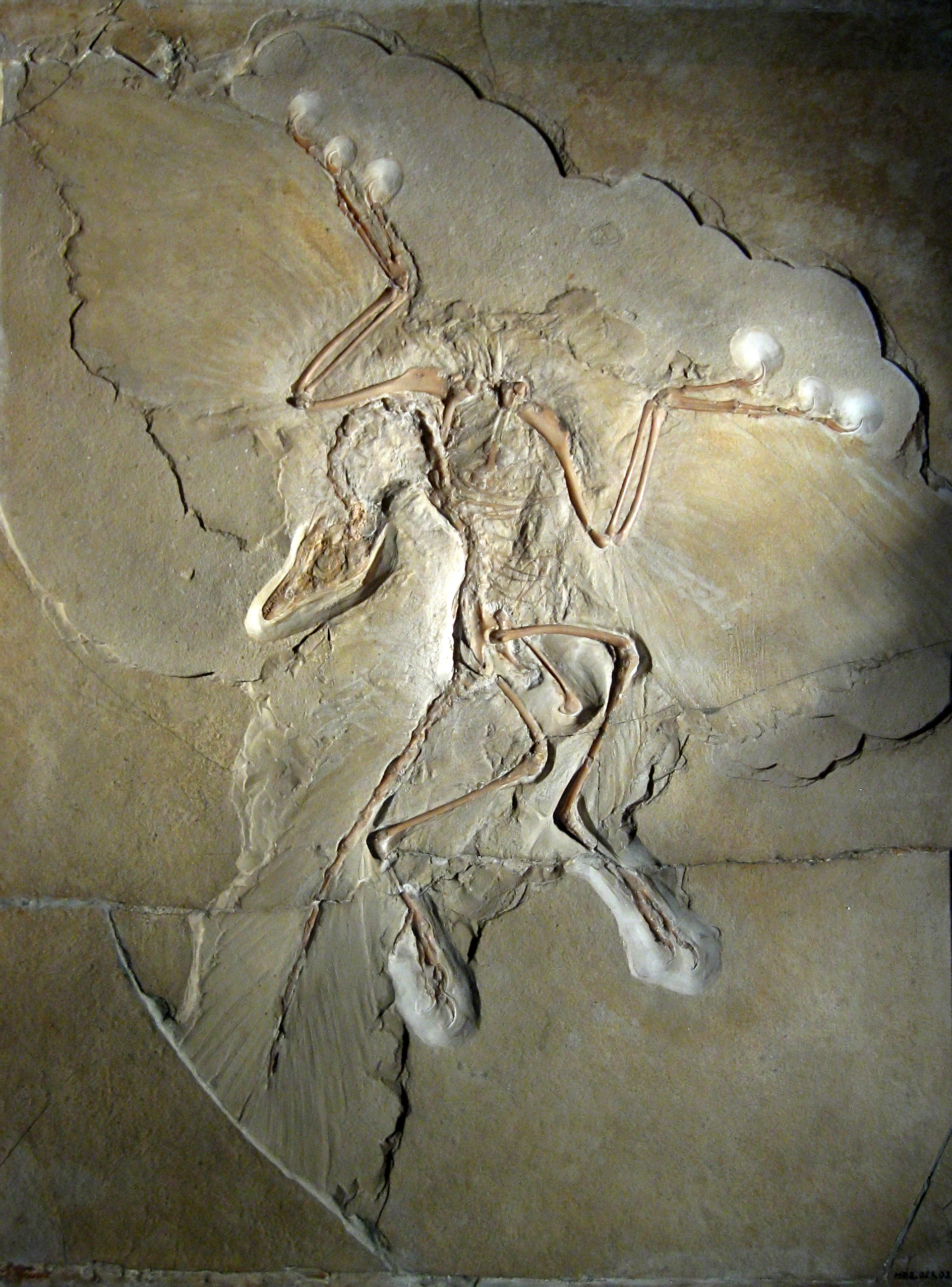
Figure 7.33: Archaeopteryx lithographica, specimen displayed at the Museum für Naturkunde in Berlin. H. Raab. 2009. CC BY-SA 3.0. https://commons.wikimedia.org/wiki/File:Archaeopteryx_lithographica_(Berlin_specimen).jpg
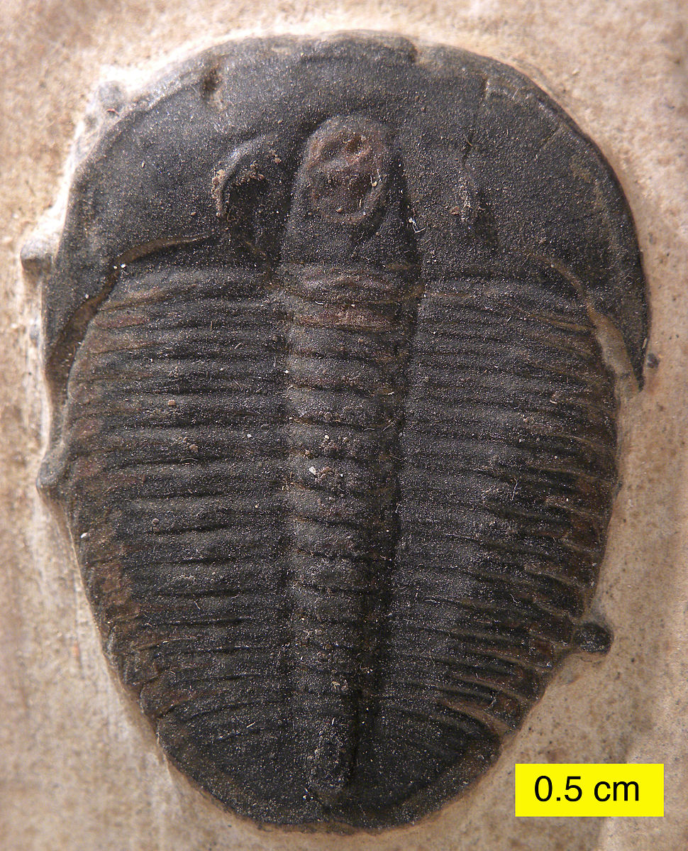
Figure 7.34: The trilobites had a hard exoskeleton, and is an early arthropod, the same group that includes modern insects, crustaceans, and arachnids. Wilson44691. 2010. Public domain. https://commons.wikimedia.org/wiki/File:ElrathiakingiUtahWheelerCambrian.jpg
Figure 7.35: Mosquito preserved in amber. Didier Desouens. 2010. CC BY-SA 4.0. https://commons.wikimedia.org/wiki/File:Ambre_Dominique_Moustique.jpg
Figure 7.36: Permineralization in petrified wood. Moondigger. 2005. CC BY-SA 2.5. https://commons.wikimedia.org/wiki/File:Petrified_forest_log_2_md.jpg
Figure 7.37: External mold of a clam. Wilson44691. 2007. Public domain. https://commons.wikimedia.org/wiki/File:Aviculopecten_subcardiformis01.JPG
Figure 7.38: Carbonized leaf. Wilson44691. 2008. Public domain. https://commons.wikimedia.org/wiki/File:ViburnumFossil.jpg
Figure 7.39: Dinosaur tracks as a record of its passing. Ballista. 2006. CC BY-SA 3.0. https://commons.wikimedia.org/wiki/File:Cheirotherium_prints_possibly_Ticinosuchus.JPG
Figure 7.40: Fossil animal droppings (coprolite). USGS. 2008. Public domain. https://commons.wikimedia.org/wiki/File:Coprolite.jpg
Figure 7.41: Variation within a population. Inglesenargentina. 2006. Public domain. https://en.wikipedia.org/wiki/File:Bell-shaped-curve.JPG
Figure 7.42: Image showing fossils that connect the continents of Gondwana (the southern continents of Pangea). Osvaldocangaspadilla. 2010. Public domain. https://commons.wikimedia.org/wiki/File:Snider-Pellegrini_Wegener_fossil_map.svg
Figure 7.43: Correlation of strata along the Grand Staircase from the Grand Canyon to Zion Canyon, Bryce Canyon, and Cedar Breaks. NPS. 2005. Public domain. https://commons.wikimedia.org/wiki/File:Grand_Staircase-big.jpg
Figure 7.44: View of Navajo Sandstone from Angel’s Landing in Zion National Park. Diliff. 2004. CC BY-SA 3.0. https://en.wikipedia.org/wiki/File:Zion_angels_landing_view.jpg
Figure 7.45: Stevens Arch in the Navajo Sandstone at Coyote Gulch some 125 miles away from Zion National Park. G. Thomas. 2007. Public domain. https://en.wikipedia.org/wiki/File:StevensArchUT.jpg
Figure 7.46: Cross-section of the Permian El Capitan Reef at Guadalupe National Monument, Texas. Kindred Grey. 2022. Adapted under fair use from Garber, R.A., Grover, G.A., & Harris, P.M. (1989). Geology of the Capitan Shelf Margin – Subsurface Data from the Northern Delaware Basin (DOI:10.2110/cor.89.13.0003).
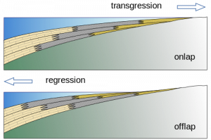
Figure 7.47: The rising sea levels of transgressions create onlapping sediments, regressions create offlapping. Woudloper. 2009. CC BY-SA 1.0. https://commons.wikimedia.org/wiki/File:Offlap_%26_onlap_EN.svg
Figure 7.48: Index fossils used for biostratigraphic correlation. David Bond. 2016. CC BY-SA 4.0. https://commons.wikimedia.org/wiki/File:Biostratigraphic_index_fossils_01.svg
Figure 7.49: Foraminifera, microscopic creatures with hard shells. Hans Hillewaert. 2011. CC BY-SA 4.0. https://en.wikipedia.org/wiki/File:Quinqueloculina_seminula.jpg
Figure 7.50: Conodonts. USGS. 2007. Public domain. https://commons.wikimedia.org/wiki/File:Conodonts.jpg
Figure 7.51: Artist reconstruction of the conodont animal. Philippe Janvier. 1997. CC BY 3.0. https://commons.wikimedia.org/wiki/File:Euconodonta.gif
Figure 7.52: Geologic time on Earth, represented circularly, to show the individual time divisions and important events. Woudloper; adapted by Hardwigg. 2010. Public domain. https://commons.wikimedia.org/wiki/File:Geologic_Clock_with_events_and_periods.svg
Figure 7.53: Geologic time scale with ages shown. USGS. 2009. Public domain. https://commons.wikimedia.org/wiki/File:Geologic_time_scale.jpg
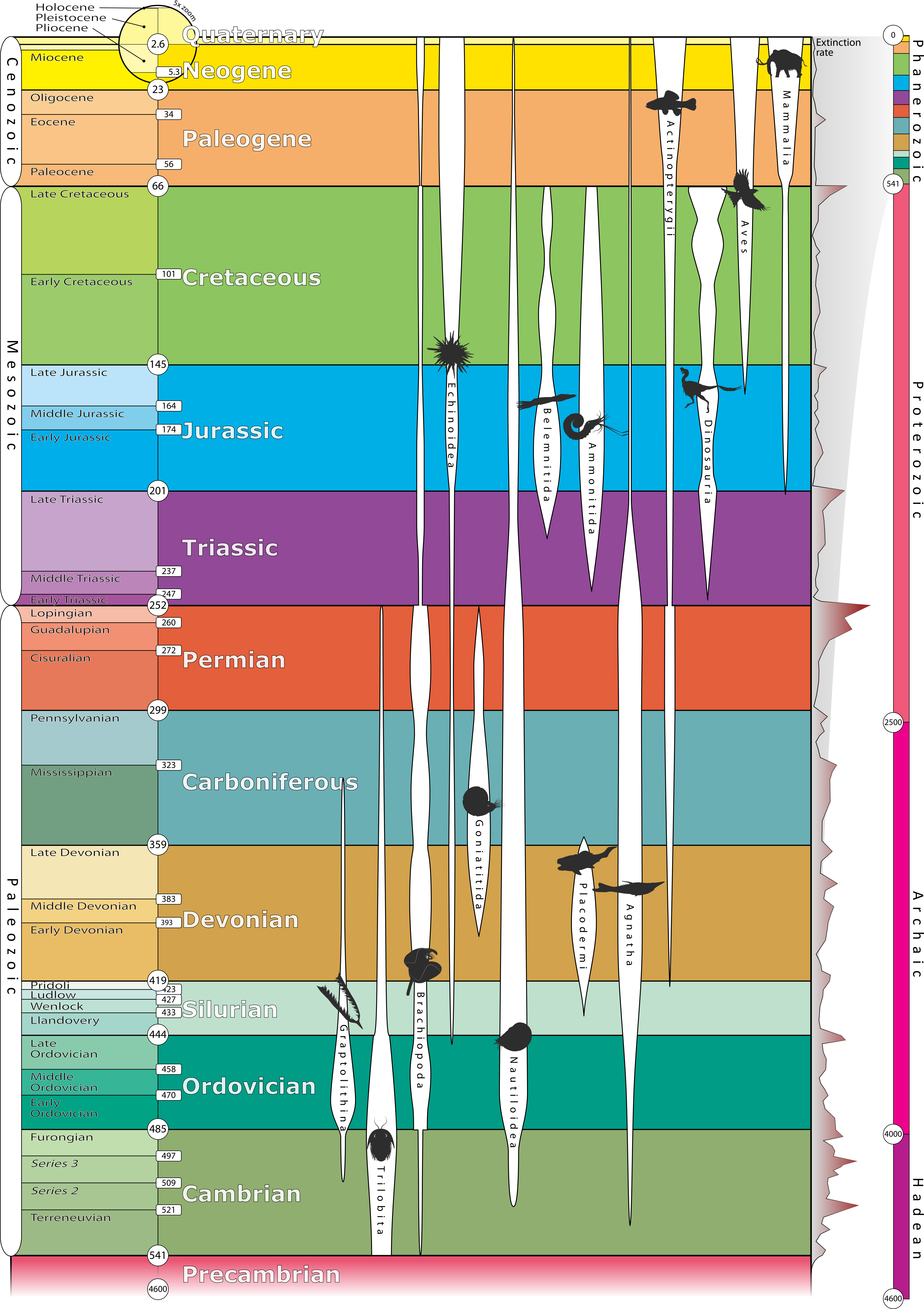
Figure 7.54: Names from the geologic time scale applied to taxonomical diversity of some major animal taxa. Frederik Lerouge. 2015. CC BY-SA 4.0. https://commons.wikimedia.org/wiki/File:Geologic_Time_Scale.png
The study of rock layers and their relationships to each other within a specific area.
Determining a qualitative age of a geologic item in relation to another geologic item.
An atom that has different number of neutrons but the same number of protons. While most properties are based on the number of protons in an element, isotopes can have subtle changes between them, including temperature fractionation and radioactivity.
Radioactive decay where two protons and two neutrons leave the isotope.
A radioactive decay process where a neutron changes into a proton, releasing an electron.
A type of radioactive decay where an electron combines with a proton, making a neutron.
The process of atoms breaking down randomly and spontaneously.
The gases that are part of the Earth, which are mainly nitrogen and oxygen.
Any evidence of ancient life.
Matching disconnected rock strata over large distances.
The largest span of time recognized by geologists, larger than an era. We are currently in the Phanerozoic eon. Rocks of a specific eon are called eonotherms.
The second largest span of time recognized by geologists; smaller than an eon, larger than a period. We are currently in the Cenozoic era.
A unit of the geologic time scale; smaller than an era, larger than an epoch. We are currently in the Quaternary period.
A type of stratigraphic correlation which is based on similar ages.
A type of stratigraphic correlation in which the physical characteristics of rocks are used to correlate.
Discernible layers of rock, typically from a sedimentary rock.
Former swamp-derived (plant) material that is part of the rock record.
Place where material is extracted from the Earth for human use.
Idea championed by James Hutton that the present is the key to the past, meaning the physical laws and processes that existed and operated in the past still exist and operate today.
In an undisturbed sequence of strata, the rocks on the bottom are older than the rocks on the top.
Layered rocks are generally laid down flat at their formation.
Pieces of rock that have been weathered and possibly eroded.
Liquid rock on the surface of the Earth.
A down-warped feature in the crust.
Layered rocks can be assumed to continue if interrupted within its area of deposition.
Place where lava is erupted at the surface.
A geologic object can not be altered until it exists, meaning, the change to the object must be younger than the object itself.
A strain that occurs in a substance in which the item changes shape due to a stress.
A rock layer that has been bent in a ductile way instead of breaking (as with faulting).
Planar feature where two blocks of bedrock move past each other via earthquakes.
Rocks that are formed from liquid rock, i.e. from volcanic processes.
An extensive, distinct, and mapped set of geologic layers.
A piece of a rock that is caught up inside of another rock.
Rocks and minerals that change within the Earth are called metamorphic, changed by heat and pressure. Metamorphism is the name of the process.
Rock more metamorphosed than phyllite, to the point that mica grains are visible. Larger porphyroblasts are sometimes present.
General name of a felsic rock that is intrusive. Has more felsic minerals than mafic minerals.
Sediment gathering together and collecting, typically in a topographic low point.
Term for the underlying lithified rocks that make up the geologic record in an area. This term can sometimes refer to only the deeper, crystalline (non-layered) rocks.
The transport and movement of weathered sediments.
Missing time in the rock record, either because of a lack of deposition and/or erosion.
Layered rocks on top of a non-layered rock, such as crystalline basement.
Two layered rocks that may seem conformable, but an erosional surface exists between them.
Angular discordance between two sets of rock layers. Caused when sedimentary strata are tilted and eroded, followed by new deposition of horizontal strata above.
Rocks that are formed by sedimentary processes, including sediments lithifying and precipitation from solution.
Places that are under ocean water at all times.
Sea level rise over time.
Sea level fall over time.
Meaning "visible life," the most recent eon in Earth's history, starting at 541 million years ago and extending through the present. Known for the diversification and evolution of life, along with the formation of Pangea.
The theory that the outer layer of the Earth (the lithosphere) is broken in several plates, and these plates move relative to one another, causing the major topographic features of Earth (e.g. mountains, oceans) and most earthquakes and volcanoes.
Rocks formed via heat and/or pressure which change the minerals within the rock.
A very high grade metamorphic rock, higher grade than schist, with a separation of light and dark minerals.
Used to describe a large mass or chain of many plutons and intrusive rocks.
Liquid rock within the Earth.
A narrow igneous intrusion that cuts through existing rock, not along bedding planes.
Place where fault movement cuts the surface of the Earth.
How smooth or rough the edges are within a sediment.
A natural substance that is typically solid, has a crystalline structure, and is typically formed by inorganic processes. Minerals are the building blocks of most rocks.
Quantitative method of dating a geologic substance or event to a specific amount of time in the past.
Initiation point of an earthquake or fault movement.
A group of all atoms with a specific number of protons, having specific, universal, and unique properties.
The calculated amount of time that half of the mass of an original (parent) radioactive isotope breaks down into a new (daughter) isotope.
An interconnected set of parts that combine and make up a whole.
The process of liquid rock solidifying into solid rock. Because liquid rock is made of many components, the process is complex as different components solidify at different temperatures.
Sedimentary rocks made of mineral grains weathered as mechanical detritus of previous rocks, e.g. sand, gravel, etc.
The rocks that existed before the changes that lead to a metamorphic rock, i.e. what rock would exist if the metamorphism was reversed.
The act of a solid coming out of solution, typically resulting from a drop in temperature or a decrease of the dissolving material.
A chemical sedimentary rock that forms as water evaporates.
Rocks (or rock textures) that are formed from explosive volcanism.
A sheet-like igneous intrusion that has intruded parallel to bedding planes within the bedrock.
ZrSiO4. Relatively chemically inert with a hardness of 8.5. Common accessory mineral in igneous and metamorphic rocks, as well as detrital sediments. Uranium can substitute for zirconium, making zircon a valuable mineral in radiometric dating.
A rock that contains material which can be turned into petroleum resources. Organic-rich muds form good source rocks.
The atom that is made after a radioactive decay.
A radioactive atom that can and will decay.
A stoney and/or metallic object from our solar system which was never incorporated into a planet and has fallen onto Earth. Meteorite is used for the rock on Earth, meteoroid for the object in space, and meteor as the object travels in Earth's atmosphere.
to move in a circular or curving course or orbit. Not to be confused with rotate, when something spins on an axis
A series of several radioactive decays which eventually leads to a stable isotope.
An atom or molecule that has a charge (positive or negative) due to the loss or gain of electrons.
A device that can determine the amounts of different isotopes in a substance.
A measure of a geologic plane's orientation in 3-D space. Used for beds of rocks, faults, fold hinges, etc. Using the right hand rule, dip is perpendicular, and to the right 90° of the strike.
When two continents crash, with no subduction (and thus little to no volcanism), since each continent is too buoyant. Many of the largest mountain ranges and broadest zones of seismic activity come from collisions.
Two or more atoms or ions that are connected chemically.
The property of unevenly-heated (heated from one direction) fluids (like water, air, ductile solids) in which warmer, less dense parts within the fluid rise while cooler, denser parts sink. This typically creates convection cells: round loops of rising and sinking material.
Middle chemical layer of the Earth, made of mainly iron and magnesium silicates. It is generally denser than the crust (except for older oceanic crust) and less dense than the core.
Breaking down rocks into small pieces by chemical or mechanical means.
Volcanic tephra that is less than 2 mm in diameter.
A specific layer of rock with identifiable properties.
Mineral group in which the silica tetrahedra, SiO4-4, is the building block.
SiO2. Transparent, but can be any color imaginable with impurities. No cleavage, hard, and commonly forms equant masses. Perfect crystals are hexagonal prisms topped with pyramidal shapes. One of the most common minerals, and is found in many different geologic settings, including the dominant component of sand on the surface of Earth. Structure is a three-dimensional network of silica tetrahedra, connected as much as possible to each other.
Average time between earthquakes calculated based on past earthquake records.
A type of non-eroded sediment mixed with organic matter, used by plants. Many essential elements for life, like nitrogen, are delivered to organisms via the soil.
Material filling in a cavity left by a organism that has dissolved away.
Organic material making a preserved impression in a rock.
The process in which solids (like minerals) are disassociated and the ionic components are dispersed in a liquid (usually water).
Depositional environments that are on land.
The fossils found at any time are unique, and the fossils in layers of different ages have progressed and changed as time has moved forward. Fossils found in layers that are not as old have organisms that more resemble organisms that are alive today.
Unchanged materials preserved in the fossil record. This is rare, and is exceedingly less likely with soft materials and older materials.
Style of fossilization where materials are replaced by minerals in groundwater fluids.
A type of fossilization where only a carbon-rich film is preserved, common in plants.
Evidence of biologic activity that is preserved in the fossil record, but it not the organism itself. Examples include footprints and burrows. Ichnology is the study of trace fossils.
Water that is below the surface.
Specialized mineralization around organic material which produces highly precise molds and casts.
Components of magma which are dissolved until it reaches the surface, where they expand. Examples include water and carbon dioxide. Volatiles also cause flux melting in the mantle, causing volcanism.
When a species no longer exists.
An accepted scientific idea that explains a process using the best available information.
A proposed explanation for an observation that can be tested.
A volcanic rock with medium silica composition, equally rich in felsic minerals (feldspar) and mafic minerals (amphibole, biotite, pyroxene). Intermediate rocks are grey in color and contain somewhat equal amounts of minerals that are light and dark in color. Primary intermediate rocks are andesite (extrusive) and diorite (intrusive).
Matching rocks of similar ages, types, etc.
A fossil with a wide geographic reach but short geologic time span used to match rock layers to a specific time period.
The mineral makeup of a rock, i.e. which minerals are found within a rock.
An interpretation of the rock record which describes the cause of sedimentation (i.e. ancient beach, river, swamp, etc.).
The part of the coastline which is directly related to water-land interaction, specifically the tidal zone and the range of wave base.
Interior body of ocean water, at least partially cut off from the main ocean water.
A topographic high found away from the beach in deeper water, but still on the continental shelf. Typically, these are formed in tropical areas by organisms such as corals.
A rock made of primarily silt.
The last period of the Paleozoic, 299-252 million years ago.
A type of stratigraphic correlation in which fossils are used to match different rock layers.
The middle period of the Mesozoic era, 201-145 million years ago.
The last period of the Mesozoic, 145-66 million years ago.
The last (and current) era of the Phanerozoic eon, starting 66 million years ago and spanning through the present.
The first period of the Paleozoic, 541 million years ago-485 million years ago.
The first period of the Mesozoic era, from 252-201 million years ago.
A chemical or biochemical rock made of mainly calcite.
A unit of geological time recognized by geologists; smaller than a period. We are currently in the Holocene epoch.
A newly-proposed time segment (an epoch) that would be representative of time since humans have changed (and left evidence behind within) the geologic record.
