11 Water
Learning Objectives
By the end of this chapter, students should be able to:
- Describe the processes of the water cycle
- Describe drainage basins, watershed protection, and water budget.
- Describe reasons for water laws, who controls them, and how water is shared in the western U.S.
- Describe zone of transport, zone of sediment production, zone of deposition, and equilibrium.
- Describe stream landforms: channel types, alluvial fans, floodplains, natural levees, deltas, entrenched meanders, and terraces.
- Describe the properties required for a good aquifer; define confining layer water table.
- Describe three major groups of water contamination and three types of remediation.
- Describe karst topography, how it is created, and the landforms that characterize it.
All life on Earth requires water. The hydrosphere (Earth’s water) is an important agent of geologic change. Water shapes our planet by depositing minerals, aiding lithification, and altering rocks after they are lithified. Water carried by subducted oceanic plates causes flux melting of upper mantle material. Water is among the volatiles in magma and emerges at the surface as steam in volcanoes.
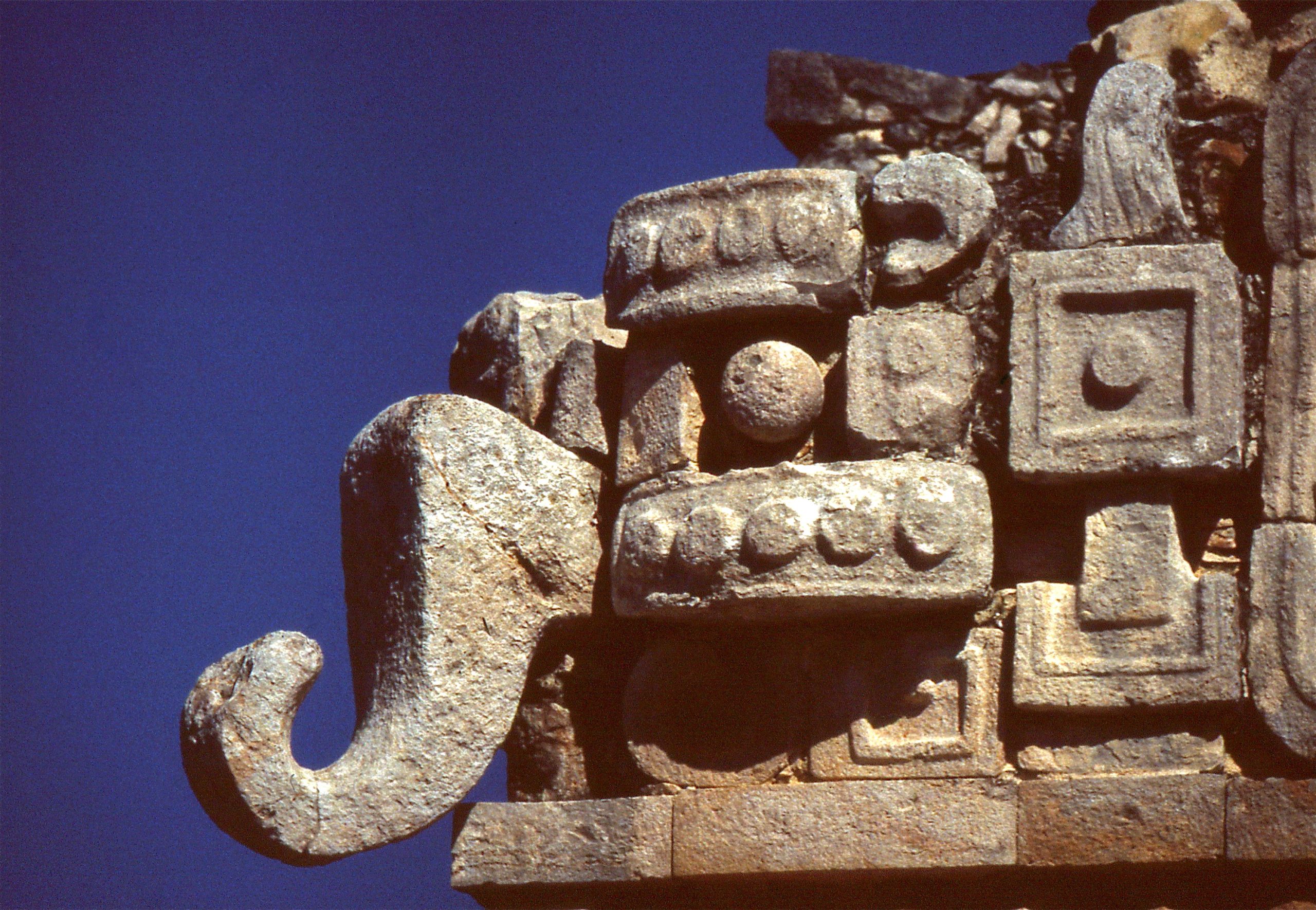
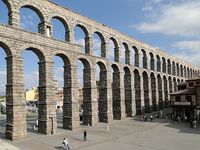
Humans rely on suitable water sources for consumption, agriculture, power generation, and many other purposes. In pre-industrial civilizations, the powerful controlled water resources. As shown in the figures, two thousand year old Roman aqueducts still grace European, Middle Eastern, and North African skylines. Ancient Mayan architecture depicts water imagery such as frogs, water-lilies, water fowl to illustrate the importance of water in their societies. In the drier lowlands of the Yucatan Peninsula, mask facades of the hooked-nosed rain god, Chac (or Chaac) are prominent on Mayan buildings such as the Kodz Poop (Temple of the Masks, sometimes spelled Coodz Poop) at the ceremonial site of Kabah. To this day government controlled water continues to be an integral part of most modern societies.
11.1 Water Cycle

The water cycle is the continuous circulation of water in the Earth’s atmosphere. During circulation, water changes between solid, liquid, and gas (water vapor) and changes location. The processes involved in the water cycle are evaporation, transpiration, condensation, precipitation, and runoff.
Evaporation is the process by which a liquid is converted to a gas. Water evaporates when solar energy warms the water sufficiently to excite the water molecules to the point of vaporization. Evaporation occurs from oceans, lakes, and streams and the land surface. Plants contribute significant amounts of water vapor as a byproduct of photosynthesis called transpiration that occurs through the minute pores of plant leaves. The term evapotranspiration refers to these two sources of water entering the atmosphere and is commonly used by geologists.
Water vapor is invisible. Condensation is the process of water vapor transitioning to a liquid. Winds carry water vapor in the atmosphere long distances. When water vapor cools or when air masses of different temperatures mix, water vapor may condense back into droplets of liquid water. These water droplets usually form around a microscopic piece of dust or salt called condensation nuclei. These small droplets of liquid water suspended in the atmosphere become visible as in a cloud. Water droplets inside clouds collide and stick together, growing into larger droplets. Once the water droplets become big enough, they fall to Earth as rain, snow, hail, or sleet.
Once precipitation has reached the Earth’s surface, it can evaporate or flow as runoff into streams, lakes, and eventually back to the oceans. Water in streams and lakes is called surface water. Or water can also infiltrate into the soil and fill the pore spaces in the rock or sediment underground to become groundwater. Groundwater slowly moves through rock and unconsolidated materials. Some groundwater may reach the surface again, where it discharges as springs, streams, lakes, and the ocean. Also, surface water in streams and lakes can infiltrate again to recharge groundwater. Therefore, the surface water and groundwater systems are connected.

Video 11.1: Water cycle.
If you are using an offline version of this text, access this YouTube video via the QR code.

Take this quiz to check your comprehension of this section.
If you are using an offline version of this text, access the quiz for section 11.1 via the QR code.
11.2 Water Basins and Budgets
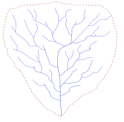
The basic unit of division of the landscape is the drainage basin, also known as a catchment or watershed. It is the area of land that captures precipitation and contributes runoff to a stream or stream segment. Drainage divides are local topographic high points that separate one drainage basin from another. Water that falls on one side of the divide goes to one stream, and water that falls on the other side of the divide goes to a different stream. Each stream, tributary and streamlet has its own drainage basin. In areas with flatter topography, drainage divides are not as easily identified but they still exist.
The headwater is where the stream begins. Smaller tributary streams combine downhill to make the larger trunk of the stream. The mouth is where the stream finally reaches its end. The mouth of most streams is at the ocean. However, a rare number of streams do not flow to the ocean, but rather end in a closed basin (or endorheic basin) where the only outlet is evaporation. Most streams in the Great Basin of Western North America end in endorheic basins. For example, in Salt Lake County, Utah, Little Cottonwood Creek and the Jordan River flow into the endorheic Great Salt Lake where the water evaporates.
Perennial streams flow all year round. Perennial streams occur in humid or temperate climates where there is sufficient rainfall and low evaporation rates. Water levels rise and fall with the seasons, depending on the discharge. Ephemeral streams flow only during rain events or the wet season. In arid climates, like Utah, many streams are ephemeral. These streams occur in dry climates with low amounts of rainfall and high evaporation rates. Their channels are often dry washes or arroyos for much of the year and their sudden flow causes flash floods.
Along Utah’s Wasatch Front, the urban area extending north to south from Brigham City to Provo, there are several watersheds that are designated as “watershed protection areas” that limit the type of use allowed in those drainages in order to protect culinary water. Dogs and swimming are limited in those watersheds because of the possibility of contamination by harmful bacteria and substances to the drinking supply of Salt Lake City and surrounding municipalities.
Water in the water cycle is very much like money in a personal budget. Income includes precipitation and stream and groundwater inflow. Expenses include groundwater withdrawal, evaporation, and stream and groundwater outflow. If the expenses outweigh the income, the water budget is not balanced. In this case, water is removed from savings, i.e. water storage, if available. Reservoirs, snow, ice, soil moisture, and aquifers all serve as storage in a water budget. In dry regions, the water is critical for sustaining human activities. Understanding and managing the water budget is an ongoing political and social challenge.
Hydrologists create groundwater budgets within any designated area, but they are generally made for watershed (basin) boundaries, because groundwater and surface water are easier to account for within these boundaries. Water budgets can be created for state, county, or aquifer extent boundaries as well. The groundwater budget is an essential component of the hydrologic model; hydrologists use measured data with a conceptual workflow of the model to better understand the water system.

Take this quiz to check your comprehension of this section.
If you are using an offline version of this text, access the quiz for section 11.2 via the QR code.
11.3 Water Use and Distribution
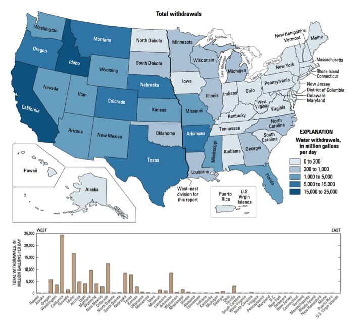
In the United States, 1,344 billion liters (355 billion gallons) of ground and surface water are used each day, of which 288 billion liters (76 billion gallons) are fresh groundwater. The state of California uses 16% of national groundwater.
Utah is the second driest state in the United States. Nevada, having a mean statewide precipitation of 31 cm (12.2 inches) per year, is the driest. Utah also has the second highest per capita rate of total domestic water use of 632.16 liters (167 gallons) per person per day. With the combination of relatively high demand and limited quantity, Utah is at risk for water budget deficits.
11.3.1 Surface Water Distribution
Fresh water is a precious resource and should not be taken for granted, especially in dry climates. Surface water makes up only 1.2% of the fresh water available on the planet, and 69% of that surface water is trapped in ground ice and permafrost. Stream water accounts for only 0.006% of all freshwater and lakes contain only 0.26% of the world’s fresh water.
Global circulation patterns are the most important factor in distributing surface water through precipitation. Due to the Coriolis effect and the uneven heating of the Earth, air rises near the equator and near latitudes 60° north and south. Air sinks at the poles and latitudes 30° north and south (see chapter 13). Land masses near rising air are more prone to humid and wet climates. Land masses near sinking air, which inhibits precipitation, are prone to dry conditions. Prevailing winds, ocean circulation patterns such as the Gulf Stream’s effects on eastern North America, rain shadows (the dry leeward sides of mountains), and even the proximity of bodies of water can affect local climate patterns. When this moist air collides with the nearby mountains causing it to rise and cool, the moisture may fall out as snow or rain on nearby areas in a phenomenon known as “lake-effect precipitation.”
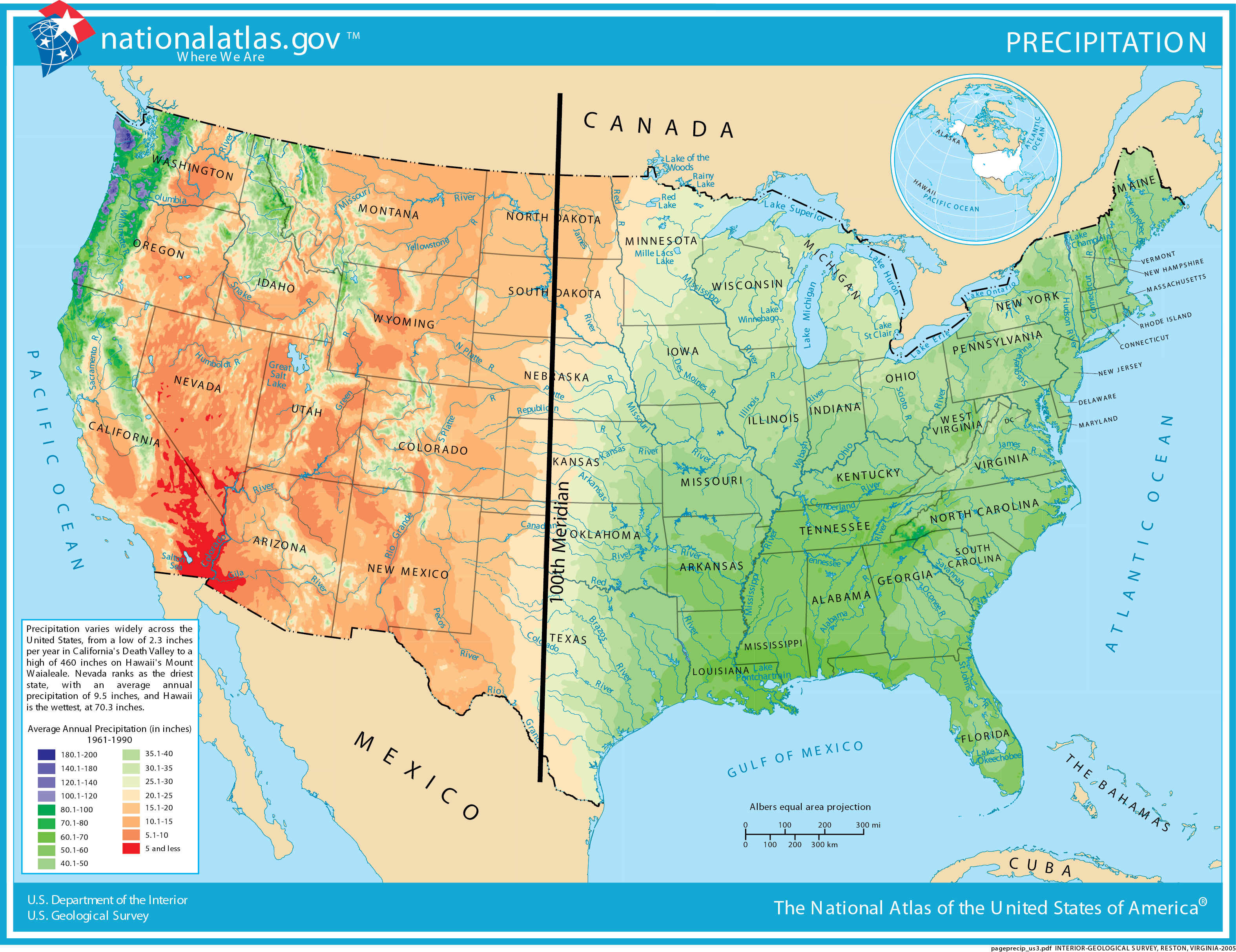
In the United States, the 100th meridian roughly marks the boundary between the humid and arid parts of the country. Growing crops west of the 100th meridian requires irrigation. In the west, surface water is stored in reservoirs and mountain snowpacks, then strategically released through a system of canals during times of high water use.
Some of the driest parts of the western United States are in the Basin and Range Province. The Basin and Range has multiple mountain ranges that are oriented north to south. Most of the basin valleys in the Basin and Range are dry, receiving less than 30 cm (12 inches) of precipitation per year. However, some of the mountain ranges can receive more than 1.52 m (60 inches) of water as snow or snow-water-equivalent. The snow-water equivalent is the amount of water that would result if the snow were melted, as the snowpack is generally much thicker than the equivalent amount of water that it would produce.
11.3.2 Groundwater Distribution
| Water source | Water volume (cubic miles) | Fresh water (%) | Total water (%) |
|---|---|---|---|
| Oceans, seas, and bays | 321,000,000 | — | 96.5% |
| Ica caps, glaciers, and permanent snow | 5,773,000 | 68.7% | 1.74% |
| Groundwater (total) | 5,614,000 | — | 1.69% |
| Groundwater (fresh) | 2,526,000 | 30.1% | 0.76% |
| Groundwater (saline) | 3,088,000 | — | 0.93% |
| Soil moisture | 3,959 | 0.05% | 0.001% |
| Ground ice and permafrost | 71,970 | 0.86% | 0.022% |
| Lakes (total) | 42,320 | — | 0.013% |
| Lakes (fresh) | 21,830 | 0.26% | 0.007% |
| Lakes (saline) | 20,490 | — | 0.006% |
| Atmosphere | 3,095 | 0.04% | 0.001% |
| Swamp water | 2,752 | 0.03% | 0.0008% |
| Rivers | 509 | 0.006% | 0.0002% |
| Biological water | 269 | 0.003% | 0.0001% |
Table 11.1: Groundwater distribution. Source: Igor Shiklomanov's chapter "World fresh water resources" in Peter H. Gleick (editor), 1993, Water in Crisis: A Guide to the World's Fresh Water Resources (Oxford University Press, New York).
Groundwater makes up 30.1% of the fresh water on the planet, making it the most abundant reservoir of fresh water accessible to most humans. The majority of freshwater, 68.7%, is stored in glaciers and ice caps as ice. As the glaciers and ice caps melt due to global warming, this fresh water is lost as it flows into the oceans.

Take this quiz to check your comprehension of this section.
If you are using an offline version of this text, access the quiz for section 11.3 via the QR code.
11.4 Water Law
Federal and state governments have put laws in place to ensure the fair and equitable use of water. In the United States, the states are tasked with creating a fair and legal system for sharing water.
11.4.1 Water Rights
Because of the limited supply of water, especially in the western United States, states disperse a system of legal water rights defined as a claim to a portion or all of a water source, such as a spring, stream, well, or lake. Federal law mandates that states control water rights, with the special exception of federally reserved water rights, such as those associated with national parks and Native American tribes, and navigation servitude that maintains navigable water bodies. Each state in the United States has a different way to disperse and manage water rights.
A person, entity, company, or organization, must have a water right to legally extract or use surface or groundwater in their state. Water rights in some western states are dictated by the concept of prior appropriation, or “first in time, first in right,” where the person with the oldest water right gets priority water use during times when there is not enough water to fulfill every water right.
The Colorado River and its tributaries pass through a desert region, including seven states (Wyoming, Colorado, Utah, New Mexico, Arizona, Nevada, California), Native American reservations, and Mexico. As the western United States became more populated and while California was becoming a key agricultural producer, the states along the Colorado River realized that the river was important to sustaining life in the West.
To guarantee certain perceived water rights, these western states recognized that a water budget was necessary for the Colorado River Basin. Thus was enacted the Colorado River Compact in 1922 to ensure that each state got a fair share of the river water. The Compact granted each state a specific volume of water based on the total measured flow at the time. However, in 1922, the flow of the river was higher than its long-term average flow, consequently, more water was allocated to each state than is typically available in the river.
Over the next several decades, lawmakers have made many other agreements and modifications regarding the Colorado River Compact, including those agreements that brought about the Hoover Dam (formerly Boulder Dam), and Glen Canyon Dam, and a treaty between the American and Mexican governments. Collectively, the agreements are referred to as “The Law of the River” by the United States Bureau of Reclamation. Despite adjustments to the Colorado River Compact, many believe that the Colorado River is still over-allocated, as the Colorado River flow no longer reaches the Pacific Ocean, its original terminus (base level). Dams along the Colorado River have caused water to divert and evaporate, creating serious water budget concerns in the Colorado River Basin. Predicted drought associated with global warming is causing additional concerns about over-allocating the Colorado River flow in the future.
The Law of the River highlights the complex and prolonged nature of interstate water rights agreements, as well as the importance of water.

Video 11.2: The Colorado River Compact of 1992.
If you are using an offline version of this text, access this YouTube video via the QR code.
The Snake Valley straddles the border of Utah and Nevada with more of the irrigable land area lying on the Utah side of the border. In 1989, the Southern Nevada Water Authority (SNWA) submitted applications for water rights to pipe up to 191,189,707 cu m (155,000 ac-ft) of water per year (an acre-foot of water is one acre covered with water one foot deep) from Spring, Snake, Delamar, Dry Lake, and Cave valleys to southern Nevada, mostly for Las Vegas. Nevada and Utah have attempted a comprehensive agreement, but negotiations have not yet been settled.

Complete this interactive activity to check your understanding.
If you are using an offline version of this text, access this interactive activity via the QR code, or by visiting https://www.arcgis.com/apps/MapJournal/index.html?appid=79199afd183e459596e6e21315159354.

If you are using an offline version of this text, access this NPR story via the QR code, or by visiting https://www.npr.org/player/embed/10953190/10956967#.

Video 11.3: Transporting Snake Valley water to satisfy a thirsty Las Vegas.
If you are using an offline version of this text, access this YouTube video via the QR code.
11.4.2 Water Quality and Protection
Two major federal laws that protect water quality in the United States are the Clean Water Act and the Safe Drinking Water Act. The Clean Water Act, an amendment of the Federal Water Pollution Control Act, protects navigable waters from dumping and point-source pollution. The Safe Drinking Water Act ensures that water that is provided by public water suppliers, like cities and towns, is safe to drink.
The U.S. Environmental Protection Agency Superfund program ensures the cleanup of hazardous contamination, and can be applied to situations of surface water and groundwater contamination. It is part of the Comprehensive Environmental Response, Compensation, and Liability Act of 1980. Under this act, state governments and the U.S. Environmental Protection Agency can use the superfund to pay for remediation of a contaminated site and then file a lawsuit against the polluter to recoup the costs. Or to avoid being sued, the polluter that caused the contamination may take direct action or provide funds to remediate the contamination.

Take this quiz to check your comprehension of this section.
If you are using an offline version of this text, access the quiz for section 11.4 via the QR code.
11.5 Surface Water
Geologically, a stream is a body of flowing surface water confined to a channel. Terms such as river, creek and brook are social terms not used in geology. Streams erode and transport sediments, making them the most important agents of the earth’s surface, along with wave action (see chapter 12) in eroding and transporting sediments. They create much of the surface topography and are an important water resource.
Several factors cause streams to erode and transport sediment, but the two main factors are stream–channel gradient and velocity. Stream–channel gradient is the slope of the stream usually expressed in meters per kilometer or feet per mile. A steeper channel gradient promotes erosion. When tectonic forces elevate a mountain, the stream gradient increases, causing the mountain stream to erode downward and deepen its channel eventually forming a valley. Stream–channel velocity is the speed at which channel water flows. Factors affecting channel velocity include channel gradient which decreases downstream, discharge and channel size which increase as tributaries coalesce, and channel roughness which decreases as sediment lining the channel walls decreases in size thus reducing friction. The combined effect of these factors is that channel velocity actually increases from mountain brooks to the mouth of the stream.
11.5.1 Discharge
Stream size is measured in terms of discharge, the volume of water flowing past a point in the stream over a defined time interval. Volume is commonly measured in cubic units (length x width x depth), shown as feet3 (ft3) or meter3 (m3). Therefore, the units of discharge are cubic feet per second (ft3/sec or cfs). Therefore, the units of discharge are cubic meters per second, (m³/s or cms, or cubic feet per second (ft³/sec or cfs). Stream discharge increases downstream. Smaller streams have less discharge than larger streams. For example, the Mississippi River is the largest river in North America, with an average flow of about 16,990.11 cms (600,000 cfs). For comparison, the average discharge of the Jordan River at Utah Lake is about 16.25 cms (574 cfs) and for the annual discharge of the Amazon River, (the world’s largest river), annual discharge is about 175,565 cms (6,200,000 cfs).
Discharge can be expressed by the following equation:
Q = V A
- Q = discharge cms (or ft3/sec),
- A = cross-sectional area of the stream channel [width times average depth] as m2 (or in2 or ft2),
- V = average channel velocity m/s (or ft/sec)
At a given location along the stream, velocity varies with stream width, shape, and depth within the stream channel as well. When the stream channel narrows but discharge remains constant, the same volume of water must flows through a narrower space causing the velocity to increase, similar to putting a thumb over the end of a backyard water hose. In addition, during rain storms or heavy snow melt, runoff increases, which increases stream discharge and velocity.
When the stream channel curves, the highest velocity will be on the outside of the bend. When the stream channel is straight and uniformly deep, the highest velocity is in the channel center at the top of the water where it is the farthest from frictional contact with the stream channel bottom and sides. In hydrology, the thalweg of a river is the line drawn that shows its natural progression and deepest channel, as is shown in the diagram.
11.5.2 Runoff versus Infiltration
Factors that dictate whether water will infiltrate into the ground or run off over the land include the amount, type, and intensity of precipitation; the type and amount of vegetation cover; the slope of the land; the temperature and aspect of the land; preexisting conditions; and the type of soil in the infiltrated area. High– intensity rain will cause more runoff than the same amount of rain spread out over a longer duration. If the rain falls faster than the soil’s properties allow it to infiltrate, then the water that cannot infiltrate becomes runoff. Dense vegetation can increase infiltration, as the vegetative cover slows the water particle’s overland flow giving them more time to infiltrate. If a parcel of land has more direct solar radiation or higher seasonal temperatures, there will be less infiltration and runoff, as evapotranspiration rates will be higher. As the land’s slope increases, so does runoff, because the water is more inclined to move downslope than infiltrate into the ground. Extreme examples are a basin and a cliff, where water infiltrates much quicker into a basin than a cliff that has the same soil properties. Because saturated soil does not have the capacity to take more water, runoff is generally greater over saturated soil. Clay-rich soil cannot accept infiltration as quickly as gravel-rich soil.
11.5.3 Drainage Patterns
The pattern of tributaries within a region is called drainage pattern. They depend largely on the type of rock beneath, and on structures within that rock (such as folds and faults). The main types of drainage patterns are dendritic, trellis, rectangular, radial, and deranged. Dendritic patterns are the most common and develop in areas where the underlying rock or sediments are uniform in character, mostly flat lying, and can be eroded equally easily in all directions. Examples are alluvial sediments or flat lying sedimentary rocks. Trellis patterns typically develop where sedimentary rocks have been folded or tilted and then eroded to varying degrees depending on their strength. The Appalachian Mountains in eastern United States have many good examples of trellis drainage. Rectangular patterns develop in areas that have very little topography and a system of bedding planes, joints, or faults that form a rectangular network. A radial pattern forms when streams flow away from a central high point such as a mountain top or volcano, with the individual streams typically having dendritic drainage patterns. In places with extensive limestone deposits, streams can disappear into the groundwater via caves and subterranean drainage and this creates a deranged pattern.
11.5.4 Fluvial Processes
Fluvial processes dictate how a stream behaves and include factors controlling fluvial sediment production, transport, and deposition. Fluvial processes include velocity, slope and gradient, erosion, transportation, deposition, stream equilibrium, and base level.
Streams can be divided into three main zones: the many smaller tributaries in the source area, the main trunk stream in the floodplain and the distributaries at the mouth of the stream. Major stream systems like the Mississippi are composed of many source areas, many tributaries and trunk streams, all coalescing into the one main stream draining the region. The zones of a stream are defined as 1) the zone of sediment production (erosion), 2) the zone of transport, and 3) the zone of deposition. The zone of sediment production is located in the headwaters of the stream. In the zone of sediment transport, there is a general balance between erosion of the finer sediment in its channel and transport of sediment across the floodplain. Streams eventually flow into the ocean or end in quiet water with a delta which is a zone of sediment deposition located at the mouth of a stream. The longitudinal profile of a stream is a plot of the elevation of the stream channel at all points along its course and illustrates the location of the three zones.
Zone of Sediment Production
The zone of sediment production is located in the headwaters of a stream where rills and gullies erode sediment and contribute to larger tributary streams. These tributaries carry sediment and water further downstream to the main trunk of the stream. Tributaries at the headwaters have the steepest gradient; erosion there produces considerable sediment carried b the stream. Headwater streams tend to be narrow and straight with small or non-existent floodplains adjacent to the channel. Since the zone of sediment production is generally the steepest part of the stream, headwaters are generally located in relatively high elevations. The Rocky Mountains of Wyoming and Colorado west of the Continental Divide contain much of the headwaters for the Colorado River which then flows from Colorado through Utah and Arizona to Mexico. Headwaters of the Mississippi river system lie east of the Continental Divide in the Rocky Mountains and west of the Appalachian Divide.
Zone of Sediment Transport
Streams transport sediment great distances from the headwaters to the ocean, the ultimate depositional basins. Sediment transportation is directly related to stream gradient and velocity. Faster and steeper streams can transport larger sediment grains. When velocity slows down, larger sediments settle to the channel bottom. When the velocity increases, those larger sediments are entrained and move again.
Transported sediments are grouped into bedload, suspended load, and dissolved load as illustrated in the above image. Sediments moved along the channel bottom are the bedload that typically consists of the largest and densest particles. Bedload is moved by saltation (bouncing) and traction (being pushed or rolled along by the force of the flow). Smaller particles are picked up by flowing water and carried in suspension as suspended load. The particle size that is carried in suspended and bedload depends on the flow velocity of the stream. Dissolved load in a stream is the total of the ions in solution from chemical weathering, including such common ions such as bicarbonate (-HCO3–), calcium (Ca+2), chloride (Cl-1), potassium (K+1), and sodium (Na+1). The amounts of these ions are not affected by flow velocity.

Video 11.4: Bed load sediment transport.
If you are using an offline version of this text, access this YouTube video via the QR code.
A floodplain is the flat area of land adjacent to a stream channel inundated with flood water on a regular basis. Stream flooding is a natural process that adds sediment to floodplains. A stream typically reaches its greatest velocity when it is close to flooding, known as the bankfull stage. As soon as the flooding stream overtops its banks and flows onto its floodplain, the velocity decreases. Sediment that was being carried by the swiftly moving water is deposited at the edge of the channel, forming a low ridge or natural levée. In addition, sediments are added to the floodplain during this flooding process contributing to fertile soils.
Zone of Sediment Deposition
Deposition occurs when bedload and suspended load come to rest on the bottom of the stream channel, lake, or ocean due to decrease in stream gradient and reduction in velocity. While both deposition and erosion occur in the zone of transport such as on point bars and cut banks, ultimate deposition where the stream reaches a lake or ocean. Landforms called deltas form where the stream enters quiet water composed of the finest sediment such as fine sand, silt, and clay.
Equilibrium and Base Level
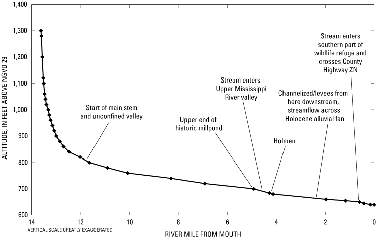
All three stream zones are present in the typical longitudinal profile of a stream which plots the elevation of the channel at all points along its course (see figure 11.14). All streams have a long profile. The long profile shows the stream gradient from headwater to mouth. All streams attempt to achieve an energetic balance among erosion, transport, gradient, velocity, discharge, and channel characteristics along the stream’s profile. This balance is called equilibrium, a state called grade.
Another factor influencing equilibrium is base level, the elevation of the stream‘s mouth representing the lowest level to which a stream can erode. The ultimate base level is, of course, sea-level. A lake or reservoir may also represent base level for a stream entering it. The Great Basin of western Utah, Nevada, and parts of some surrounding states contains no outlets to the sea and provides internal base levels for streams within it. Base level for a stream entering the ocean changes if sea-level rises or falls. Base level also changes if a natural or human-made dam is added along a stream‘s profile. When base level is lowered, a stream will cut down and deepen its channel. When base level rises, deposition increases as the stream adjusts attempting to establish a new state of equilibrium. A stream that has approximately achieved equilibrium is called a graded stream.
11.5.5 Fluvial Landforms
Stream landforms are the land features formed on the surface by either erosion or deposition. The stream-related landforms described here are primarily related to channel types.
Channel Types
Stream channels can be straight, braided, meandering, or entrenched. The gradient, sediment load, discharge, and location of base level all influence channel type. Straight channels are relatively straight, located near the headwaters, have steep gradients, low discharge, and narrow V-shaped valleys. Examples of these are located in mountainous areas.
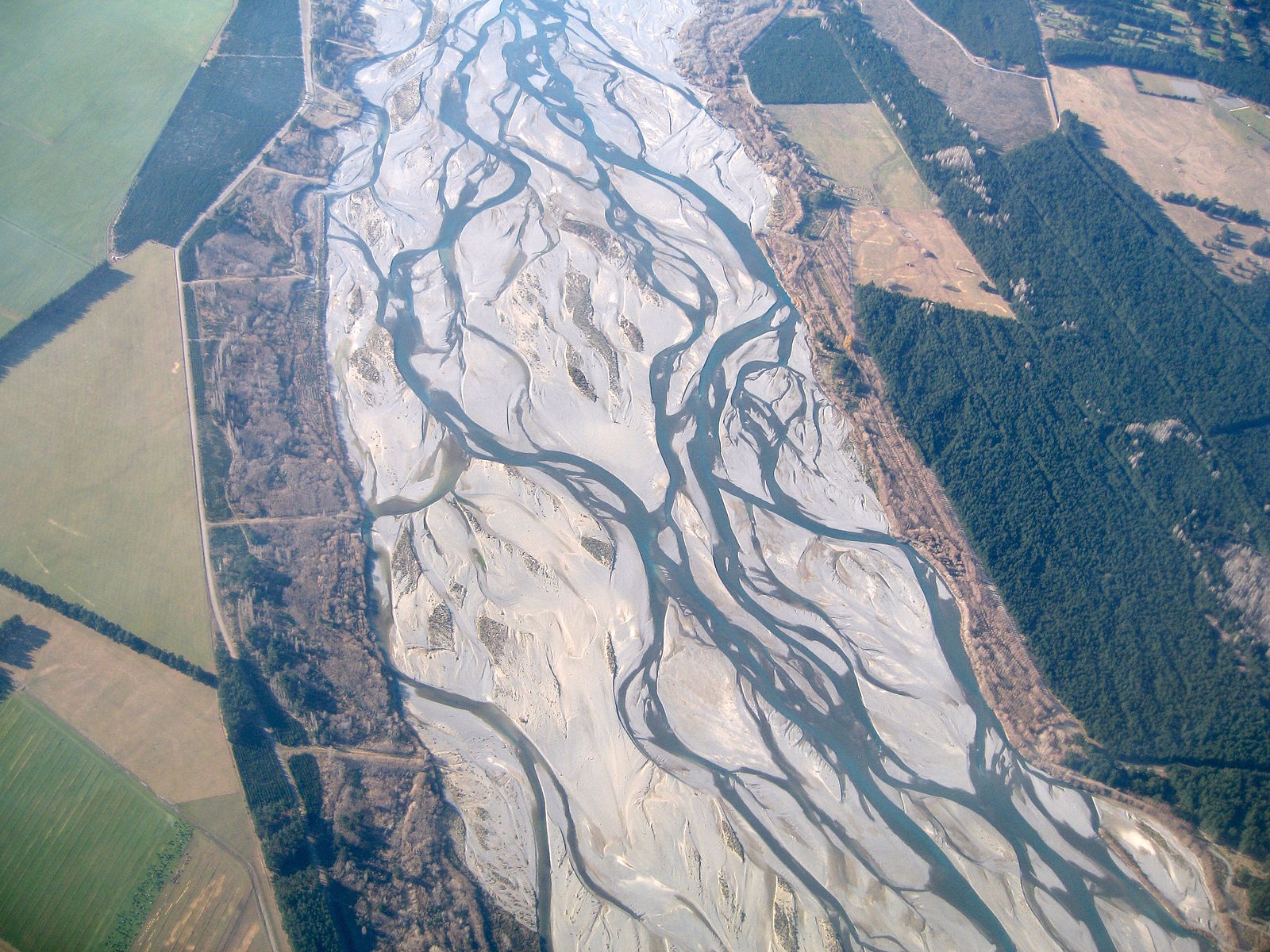
Braided streams have multiple channels splitting and recombining around numerous mid-channel bars. These are found in floodplains with low gradients in areas with near sources of coarse sediment such as trunk streams draining mountains or in front of glaciers.
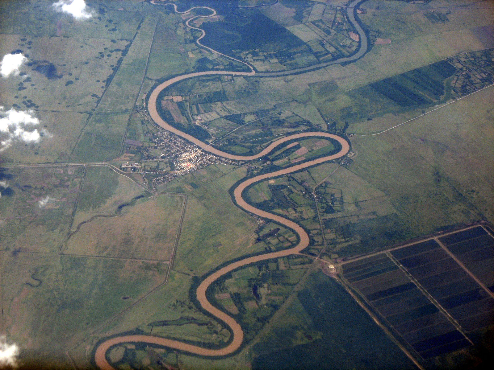
Meandering streams have a single channel that curves back and forth like a snake within its floodplain where it emerges from its headwaters into the zone of transport. Meandering streams are dynamic creating a wide floodplain by eroding and extending meander loops side-to-side. The highest velocity water is located on the outside of a meander bend. Erosion of the outside of the curve creates a feature called a cut bank and the meander extends its loop wider by this erosion.
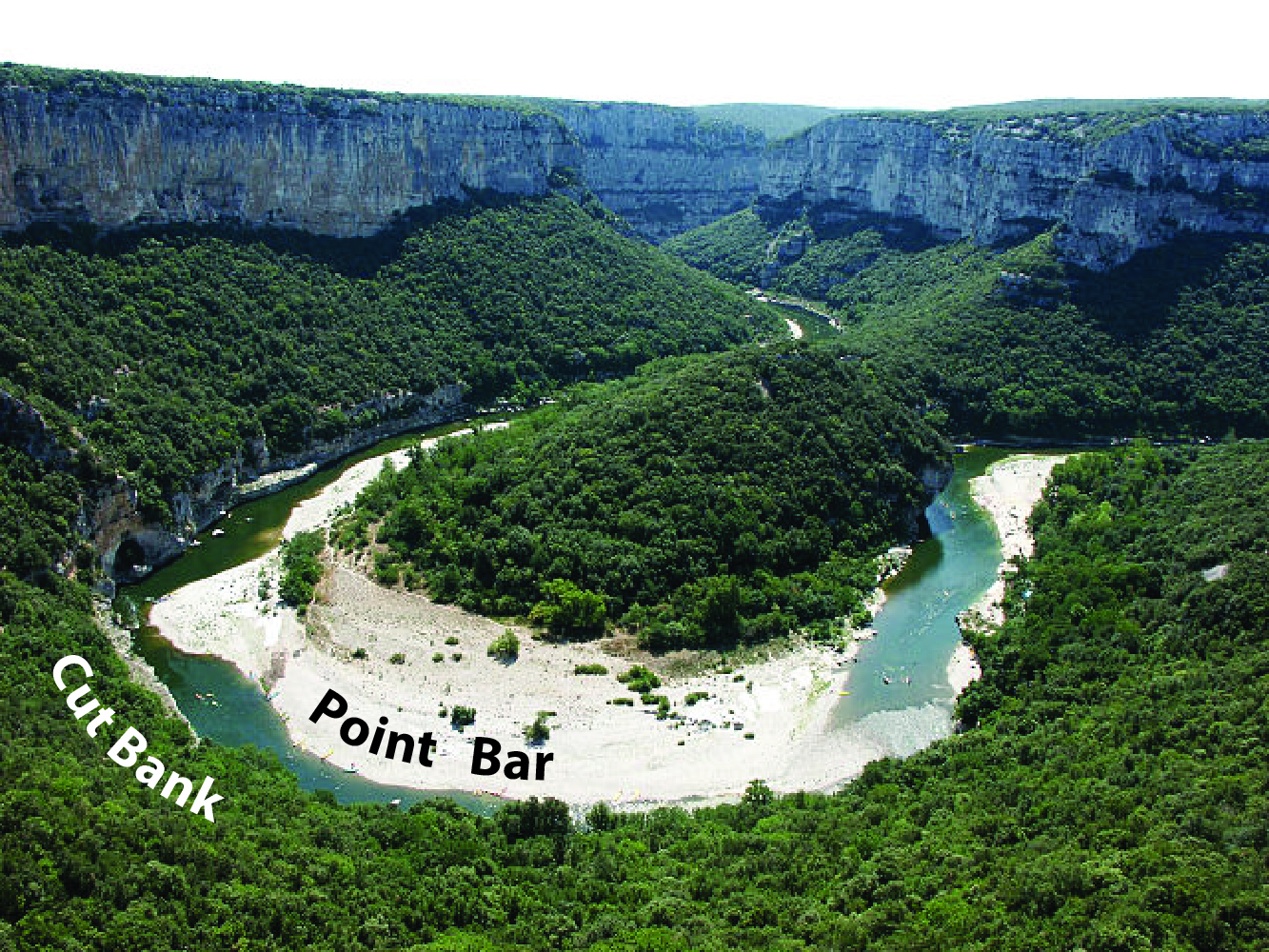
The thalweg of the stream is the deepest part of the stream channel. In the straight parts of the channel, the thalweg and highest velocity are in the center of the channel. But at the bend of a meandering stream, the thalweg shifts toward the cut bank. Opposite the cutbank on the inside bend of the channel is the lowest stream velocity and is an area of deposition called a point bar.
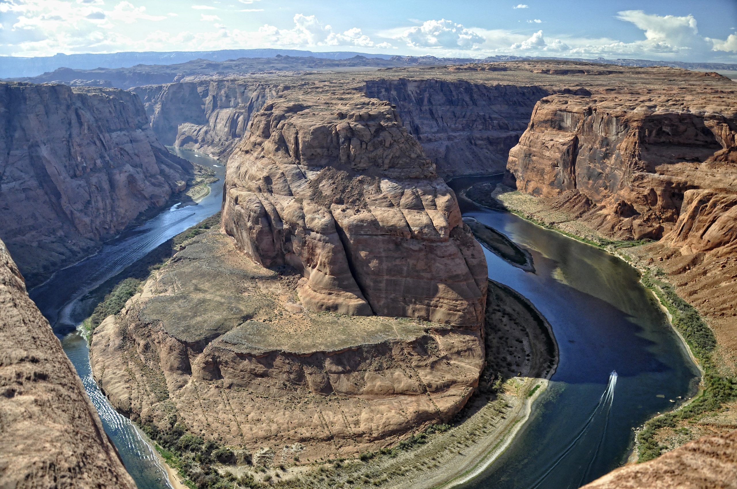
In areas of tectonic uplift such as on the Colorado Plateau, meandering streams that once flowed on the plateau surface have become entrenched or incised as uplift occurred and the stream cut its meandering channel down into bedrock. Over the past several million years, the Colorado River and its tributaries have incised into the flat lying rocks of the plateau by hundreds, even thousands of feet creating deep canyons including the Grand Canyon in Arizona.
Many fluvial landforms occur on a floodplain associated with a meandering stream. Meander activity and regular flooding contribute to widening the floodplain by eroding adjacent uplands. The stream channels are confined by natural levees that have been built up over many years of regular flooding. Natural levees can isolate and direct flow from tributary channels on the floodplain from immediately reaching the main channel. These isolated streams are called yazoo streams and flow parallel to the main trunk stream until there is an opening in the levee to allow for a belated confluence.

Video 11.5: How is a levee formed?
If you are using an offline version of this text, access this YouTube video via the QR code.
To limit flooding, humans build artificial levees on flood plains. Sediment that breaches the levees during flood stage is called crevasse splays and delivers silt and clay onto the floodplain. These deposits are rich in nutrients and often make good farm land. When floodwaters crest over human-made levees, the levees quickly erode with potentially catastrophic impacts. Because of the good soils, farmers regularly return after floods and rebuild year after year.
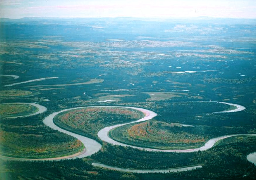
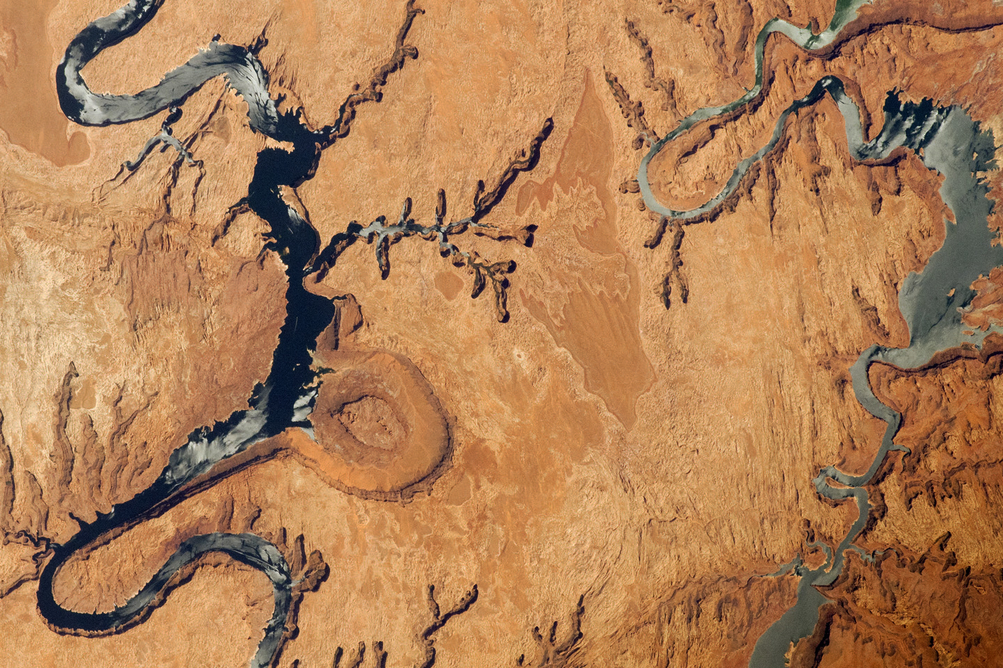
Through erosion on the outsides of the meanders and deposition on the insides, the channels of meandering streams move back and forth across their floodplain over time. On very broad floodplains with very low gradients, the meander bends can become so extreme that they cut across themselves at a narrow neck (see figure 11.22) called a cutoff. The former channel becomes isolated and forms an oxbow lake seen on the right of the figure. Eventually the oxbow lake fills in with sediment and becomes a wetland and eventually a meander scar. Stream meanders can migrate and form oxbow lakes in a relatively short amount of time. Where stream channels form geographic and political boundaries, this shifting of channels can cause conflicts.

Video 11.6: Why do rivers curve?
If you are using an offline version of this text, access this YouTube video via the QR code.
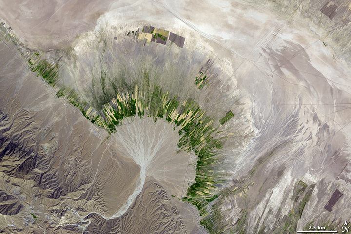
Alluvial fans are a depositional landform created where streams emerge from mountain canyons into a valley. The channel that had been confined by the canyon walls is no longer confined, slows down and spreads out, dropping its bedload of all sizes, forming a delta in the air of the valley. As distributary channels fill with sediment, the stream is diverted laterally, and the alluvial fan develops into a cone shaped landform with distributaries radiating from the canyon mouth. Alluvial fans are common in the dry climates of the West where ephemeral streams emerge from canyons in the ranges of the Basin and Range.

Complete this interactive activity to check your understanding.
If you are using an offline version of this text, access this interactive activity via the QR code.
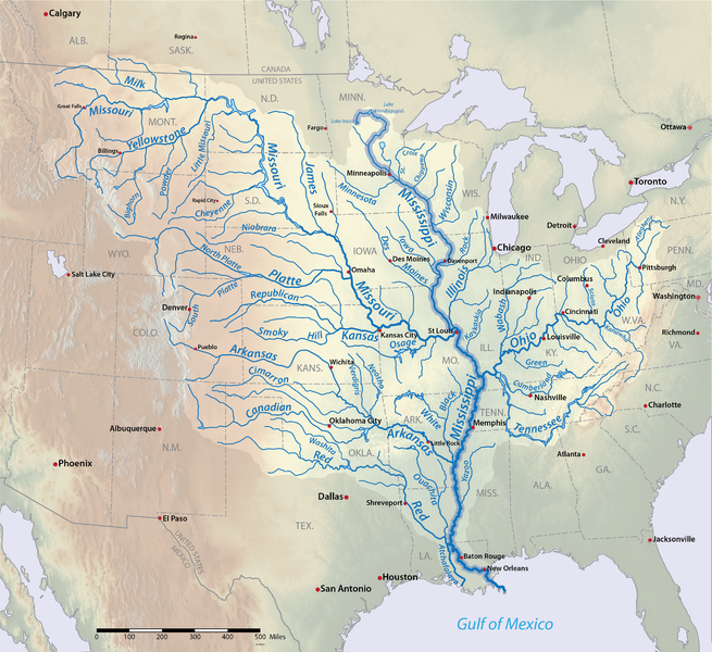
A delta is formed when a stream reaches a quieter body of water such as a lake or the ocean and the bedload and suspended load is deposited. If wave erosion from the water body is greater than deposition from the river, a delta will not form. The largest and most famous delta in the United States is the Mississippi River delta formed where the Mississippi River flows into the Gulf of Mexico. The Mississippi River drainage basin is the largest in North America, draining 41% of the contiguous United States. Because of the large drainage area, the river carries a large amount of sediment. The Mississippi River is a major shipping route and human engineering has ensured that the channel has been artificially straightened and remains fixed within the floodplain. The river is now 229 km shorter than it was before humans began engineering it. Because of these restraints, the delta is now focused on one trunk channel and has created a “bird’s foot” pattern. The two NASA images below of the delta show how the shoreline has retreated and land was inundated with water while deposition of sediment was focused at end of the distributaries. These images have changed over a 25 year period from 1976 to 2001. These are stark changes illustrating sea-level rise and land subsidence from the compaction of peat due to the lack of sediment resupply.

Complete this interactive activity to check your understanding.
If you are using an offline version of this text, access this interactive activity via the QR code.
The formation of the Mississippi River delta started about 7500 years ago when postglacial sea level stopped rising. In the past 7000 years, prior to anthropogenic modifications, the Mississippi River delta formed several sequential lobes. The river abandoned each lobe for a more preferred route to the Gulf of Mexico. These delta lobes were reworked by the ocean waves of the Gulf of Mexico. After each lobe was abandoned by the river, isostatic depression and compaction of the sediments caused basin subsidence and the land to sink.
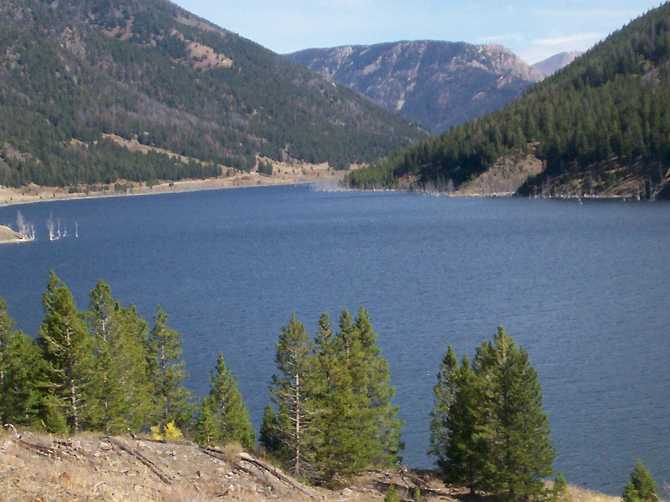
A clear example of how deltas form came from an earthquake. During the 1959 Madison Canyon 7.5 magnitude earthquake in Montana, a large landslide dammed the Madison River forming Quake Lake still there today. A small tributary stream that once flowed into the Madison River, now flows into Quake Lake forming a delta composed of coarse sediment actively eroded from the mountainous upthrown block to the north.
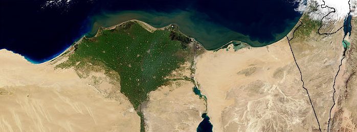
Deltas can be further categorized as wave-dominated or tide-dominated. Wave-dominated deltas occur where the tides are small and wave energy dominates. An example is the Nile River delta in the Mediterranean Sea that has the classic shape of the Greek character (Δ) from which the landform is named. A tide-dominated delta forms when ocean tides are powerful and influence the shape of the delta. For example, Ganges-Brahmaputra Delta in the Bay of Bengal (near India and Bangladesh) is the world’s largest delta and mangrove swamp called the Sundarban.
At the Sundarban Delta in Bangladesh, tidal forces create linear intrusions of seawater into the delta. This delta also holds the world’s largest mangrove swamp.
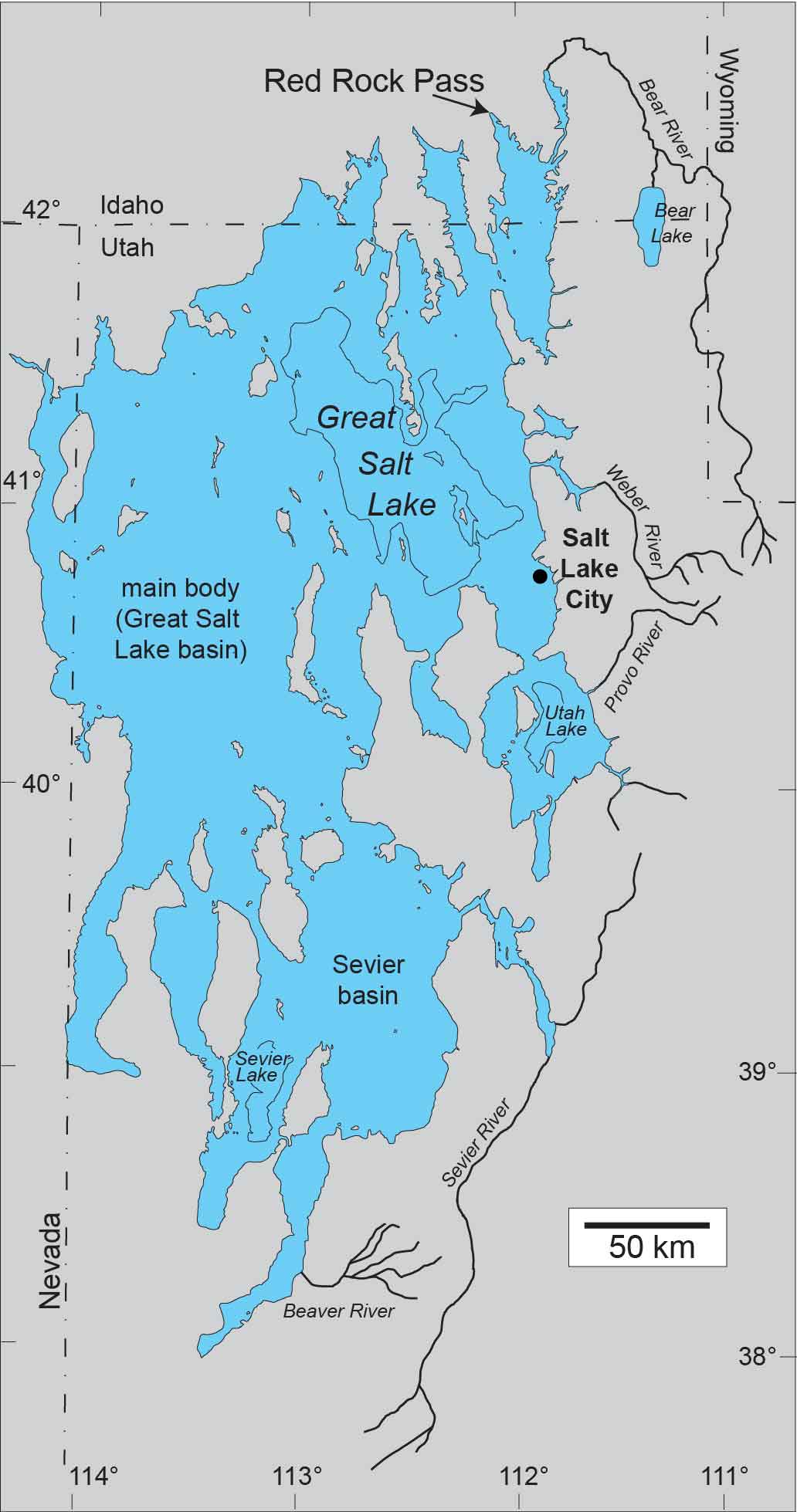
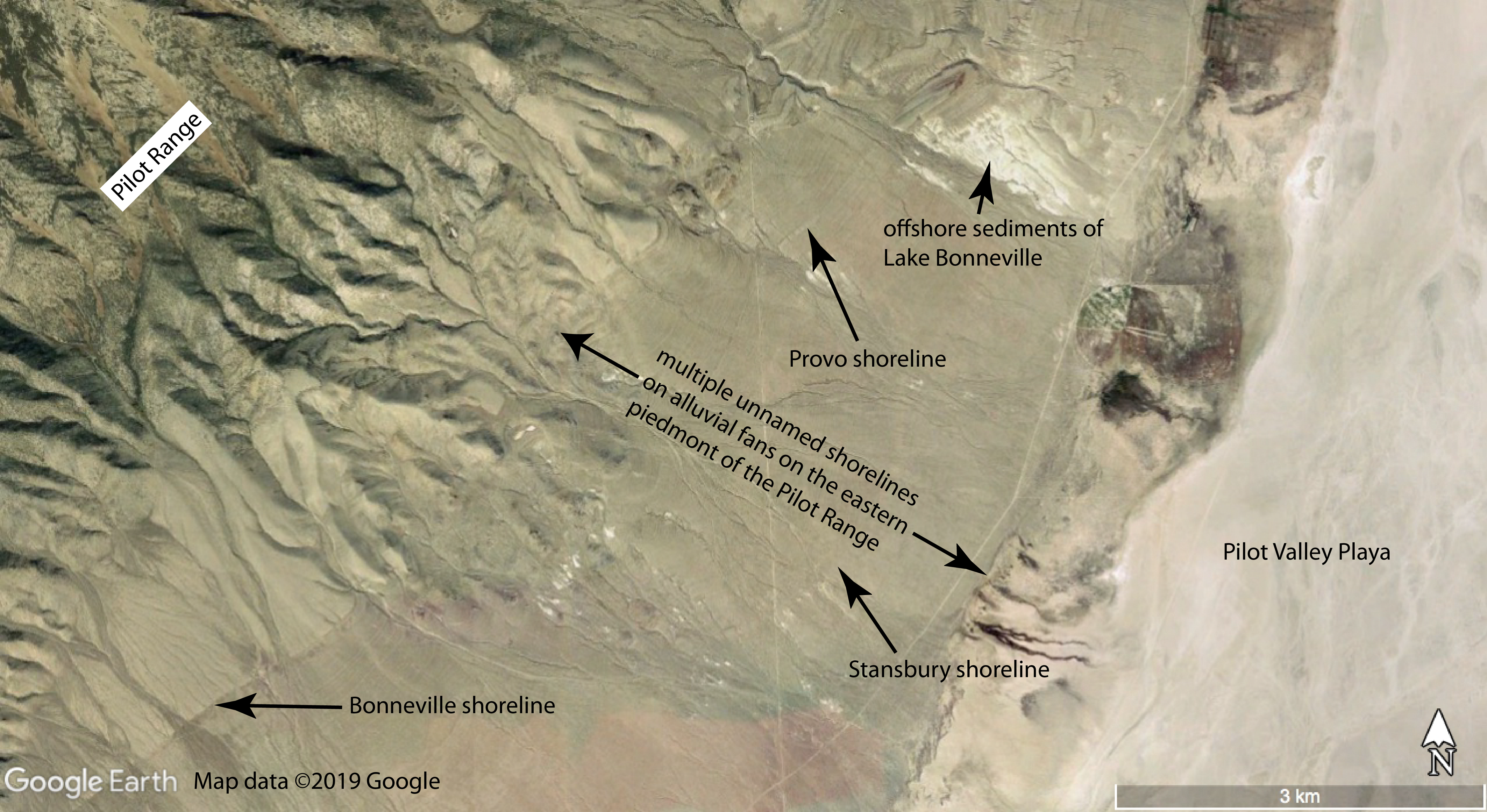
Lake Bonneville was a large, pluvial lake that occupied the western half of Utah and parts of eastern Nevada from about 30,000 to 12,000 years ago. The lake filled to a maximum elevation as great as approximately 5100 feet above mean sea level, filling the basins, leaving the mountains exposed, many as islands. The presence of the lake allowed for deposition of both fine grained lake mud and silt and coarse gravels from the mountains. Variations in lake level were controlled by regional climate and a catastrophic failure of Lake Bonneville’s main outlet, Red Rock Pass. During extended periods of time in which the lake level remained stable, wave-cut terraces were produced that can be seen today on the flanks of many mountains in the region. Significant deltas formed at the mouths of major canyons in Salt Lake, Cache, and other Utah valleys. The Great Salt Lake is the remnant of Lake Bonneville and cities have built up on these delta deposits.
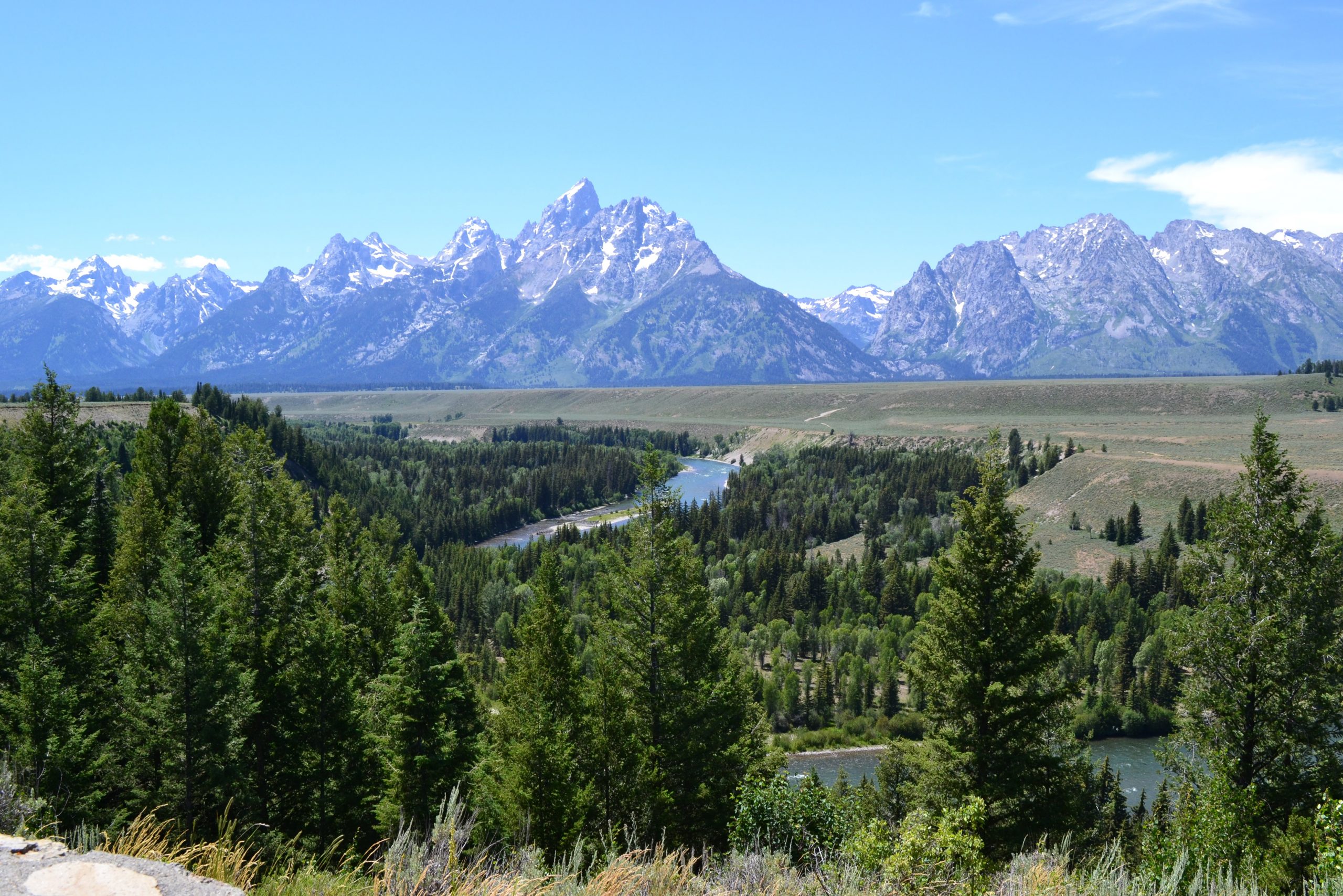
Stream terraces are remnants of older floodplains located above the existing floodplain and river. Like entrenched meanders, stream terraces form when uplift occurs or base level drops and streams erode downward, their meanders widening a new flood plain. Stream terraces can also form from extreme flood events associated with retreating glaciers. A classic example of multiple stream terraces are along the Snake River in Grand Teton National Park in Wyoming.

Take this quiz to check your comprehension of this section.
If you are using an offline version of this text, access the quiz for section 11.5 via the QR code.
11.6 Groundwater
Groundwater is an important source of freshwater. It can be found at varying depths in all places under the ground, but is limited by extractable quantity and quality.

Video 11.7: What is an aquifer?
If you are using an offline version of this text, access this YouTube video via the QR code.
11.6.1 Porosity and Permeability
An aquifer is a rock unit that contains extractable ground water. A good aquifer must be both porous and permeable. Porosity is the space between grains that can hold water, expressed as the percentage of open space in the total volume of the rock. Permeability comes from connectivity of the spaces that allows water to move in the aquifer. Porosity can occur as primary porosity, as space between sand grains or vesicles in volcanic rocks, or secondary porosity as fractures or dissolved spaces in rock). Compaction and cementation during lithification of sediments reduces porosity (see section 5.3).
A combination of a place to contain water (porosity) and the ability to move water (permeability) makes a good aquifer—a rock unit or sediment that allows extraction of groundwater. Well-sorted sediments have higher porosity because there are not smaller sediment particles filling in the spaces between the larger particles. Shales made of clays generally have high porosity, but the pores are poorly connected, thereby causing low permeability.

Video 11.8: Porosity and permeability.
If you are using an offline version of this text, access this YouTube video via the QR code.
While permeability is an important measure of a porous material’s ability to transmit water, hydraulic conductivity is more commonly used by geologists to measure how easily a fluid is transmitted. Hydraulic conductivity measures both the permeability of the porous material and the properties of the water, or whatever fluid is being transmitted like oil or gas. Because hydraulic conductivity also measures the properties of the fluid, such as viscosity, it is used by both petroleum geologists and hydrogeologists to describe both the production capability of oil reservoirs and of aquifers. High hydraulic conductivity indicates that fluid transmits rapidly through an aquifer.
11.6.2 Aquifers
Aquifers are rock layers with sufficient porosity and permeability to allow water to be both contained and move within them. For rock or sediment to be considered an aquifer, its pores must be at least partially filled with water and it must be permeable enough to transmit water. Drinking water aquifers must also contain potable water. Aquifers can vary dramatically in scale, from spanning several formations covering large regions to being a local formation in a limited area. Aquifers adequate for water supply are both permeable, porous, and potable.
11.6.3 Groundwater Flow
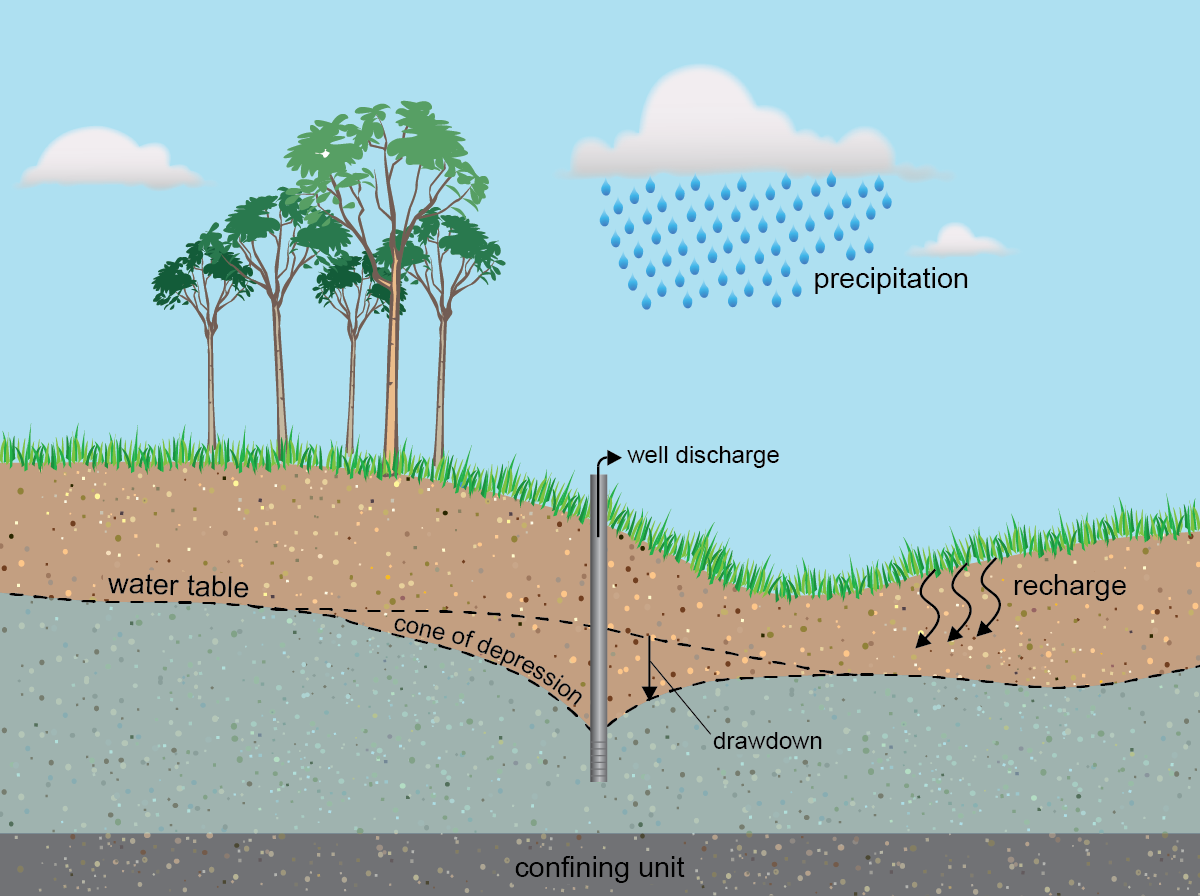
When surface water infiltrates or seeps into the ground, it usually enters the unsaturated zone also called the vadose zone, or zone of aeration. The vadose zone is the volume of geologic material between the land surface and the zone of saturation where the pore spaces are not completely filled with water. Plant roots inhabit the upper vadose zone and fluid pressure in the pores is less than atmospheric pressure. Below the vadose zone is the capillary fringe. Capillary fringe is the usually thin zone below the vadose zone where the pores are completely filled with water (saturation), but the fluid pressure is less than atmospheric pressure. The pores in the capillary fringe are filled because of capillary action, which occurs because of a combination of adhesion and cohesion. Below the capillary fringe is the saturated zone or phreatic zone, where the pores are completely saturated and the fluid in the pores is at or above atmospheric pressure. The interface between the capillary fringe and the saturated zone marks the location of the water table.
Wells are conduits that extend into the ground with openings to the aquifers, to extract from, measure, and sometimes add water to the aquifer. Wells are generally the way that geologists and hydrologist measure the depth to groundwater from the land surface as well as withdraw water from aquifers.
Water is found throughout the pore spaces in sediments and bedrock. The water table is the area below which the pores are fully saturated with water. The simplest case of a water table is when the aquifer is unconfined, meaning it does not have a confining layer above it. Confining layers can pressurize aquifers by trapping water that is recharged at a higher elevation underneath the confining layer, allowing for a potentiometric surface higher than the top of the aquifer, and sometimes higher than the land surface.
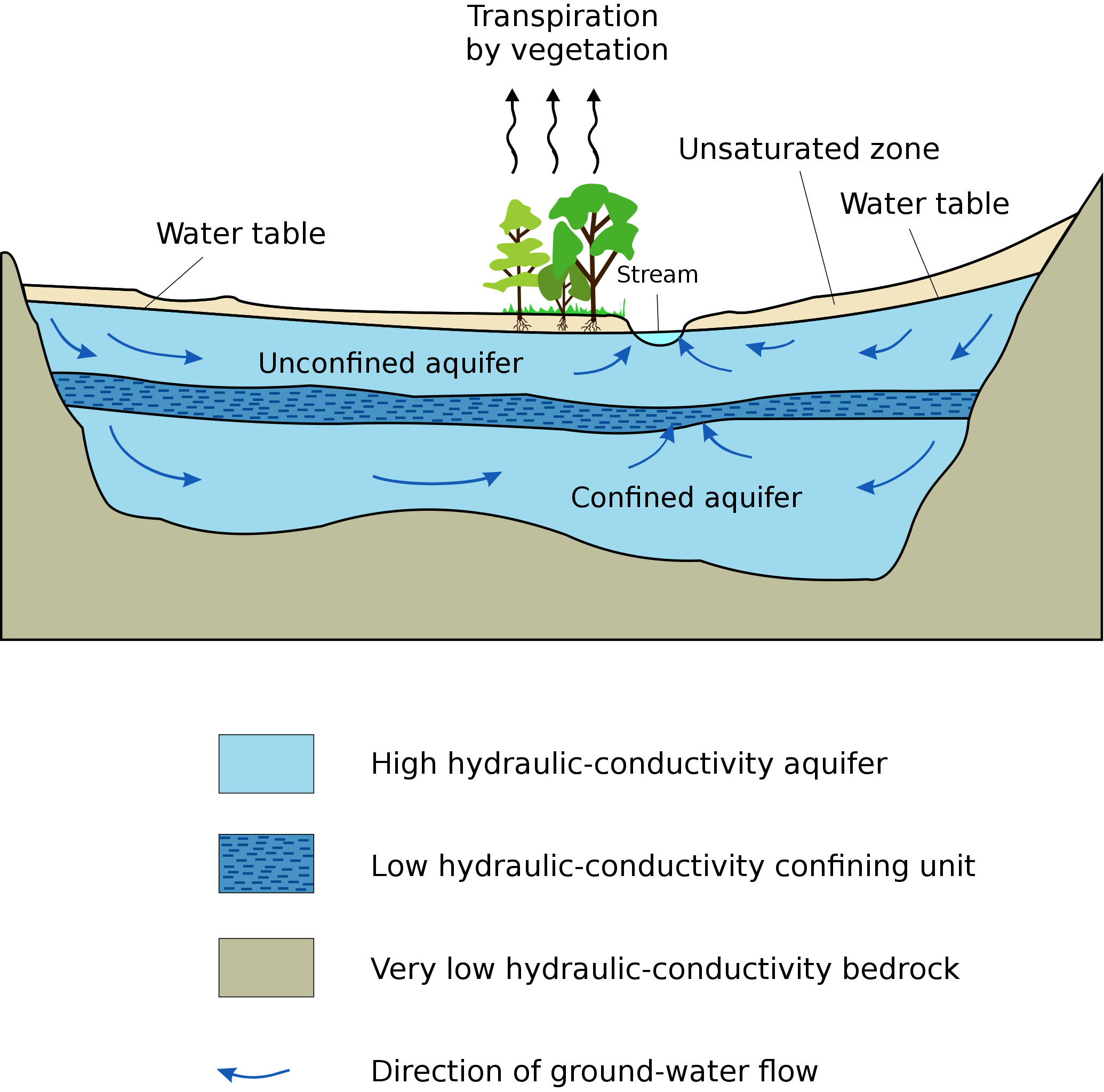
A confining layer is a low permeability layer above and/or below an aquifer that restricts the water from moving in and out of the aquifer. Confining layers include aquicludes, which are so impermeable that no water travels through them, and aquitards, which significantly decrease the speed at which water travels through them. The potentiometric surface represents the height that water would rise in a well penetrating the pressurized aquifer system. Breaches in the pressurized aquifer system, like faults or wells, can cause springs or flowing wells, also known as artesian wells.
The water table will generally mirror surface topography, though more subdued, because hydrostatic pressure is equal to atmospheric pressure along the surface of the water table. If the water table intersects the ground surface the result will be water at the surface in the form of a gaining stream, spring, lake, or wetland. The water table intersects the channel for gaining streams which then gains water from the water table. The channels for losing streams lie below the water table, thus losing streams lose water to the water table. Losing streams may be seasonal during a dry season or ephemeral in dry climates where they may normally be dry and carry water only after rain storms. Ephemeral streams pose a serious danger of flash flooding in dry climates.

Video 11.9: Where is the water table?
If you are using an offline version of this text, access this YouTube video via the QR code.
Mentioned in the video is the USGS Groundwater Watch site.
Using wells, geologists measure the water table’s height and the potentiometric surface. Graphs of the depth to groundwater over time, are known as hydrographs and show changes in the water table over time. Well–water level is controlled by many factors and can change very frequently, even every minute, seasonally, and over longer periods of time.
In 1856, French engineer Henry Darcy developed a hypothesis to show how discharge through a porous medium is controlled by permeability, pressure, and cross–sectional area. To prove this relationship, Darcy experimented with tubes of packed sediment with water running through them. The results of his experiments empirically established a quantitative measure of hydraulic conductivity and discharge that is known as Darcy’s law. The relationships described by Darcy’s Law have close similarities to Fourier’s law in the field of heat conduction, Ohm’s law in the field of electrical networks, or Fick’s law in diffusion theory.
Q=KA(Δh/L)
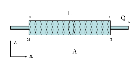
- Q = flow (volume/time)
- K = hydraulic conductivity (length/time)
- A = cross-sectional area of flow (area)
- Δh = change in pressure head (pressure difference)
- L = distance between pressure (h) measurements (length)
- Δh/L is commonly referred to as the hydraulic gradient
Pumping water from an unconfined aquifer lowers the water table. Pumping water from a confined aquifer lowers the pressure and/or potentiometric surface around the well. In an unconfined aquifer, the water table is lowered as water is removed from the aquifer near the well producing drawdown and a cone of depression (see figure 11.34). In a confined aquifer, pumping on an artesian well reduces the pressure or potentiometric surface around the well.
When one cone of depression intersects another cone of depression or a barrier feature like an impermeable mountain block, drawdown is intensified. When a cone of depression intersects a recharge zone, the cone of depression is lessened.
11.6.4 Recharge
The recharge area is where surface water enters an aquifer through the process of infiltration. Recharge areas are generally topographically high locations of an aquifer. They are characterized by losing streams and permeable rock that allows infiltration into the aquifer. Recharge areas mark the beginning of groundwater flow paths.
In the Basin and Range Province, recharge areas for the unconsolidated aquifers of the valleys are along mountain foothills. In the foothills of Salt Lake Valley, losing streams contribute water to the gravel-rich deltaic deposits of ancient Lake Bonneville, in some cases feeding artesian wells in the Salt Lake Valley.
An aquifer management practice is to induce recharge through storage and recovery. Geologists and hydrologists can increase the recharge rate into an aquifer system using injection wells and infiltration galleries or basins. Injection wells pump water into an aquifer where it can be stored. Injection wells are regulated by state and federal governments to ensure that the injected water is not negatively impacting the quality or supply of the existing groundwater in the aquifer. Some aquifers can store significant quantities of water, allowing water managers to use the aquifer system like a surface reservoir. Water is stored in the aquifer during periods of low water demand and high water supply and later extracted during times of high water demand and low water supply.
11.6.5 Discharge
Discharge areas are where the water table or potentiometric surface intersects the land surface. Discharge areas mark the end of groundwater flow paths. These areas are characterized by springs, flowing (artesian) wells, gaining streams, and playas in the dry valley basins of the Basin and Range Province of the western United States.
11.6.6 Groundwater Mining and Subsidence
Like other natural resources on our planet, the quantity of fresh and potable water is finite. The only natural source of water on land is from the sky in the form of precipitation. In many places, groundwater is being extracted faster than it is being replenished. When groundwater is extracted faster than it is recharged, groundwater levels and potentiometric surfaces decline, and discharge areas diminish or dry up completely. Regional pumping-induced groundwater decline is known as groundwater mining or groundwater overdraft. Groundwater mining is a serious situation and can lead to dry wells, reduced spring and stream flow, and subsidence. Groundwater mining is happening is places where more water is extracted by pumping than is being replenished by precipitation, and the water table is continually lowered. In these situations, groundwater must be viewed as a ore body and in its depletion, the possibility of producing ghost towns.

Video 11.10: Groundwater.
If you are using an offline version of this text, access this YouTube video via the QR code.
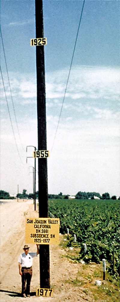
In many places, water actually helps hold up an aquifer’s skeleton by the water pressure exerted on the grains in an aquifer. This pressure is called pore pressure and comes from the weight of overlying water. If pore pressure decreases because of groundwater mining, the aquifer can compact, causing the surface of the ground to sink. Areas especially susceptible to this effect are aquifers made of unconsolidated sediments. Unconsolidated sediments with multiple layers of clay and other fine-grained material are at higher risk because when water is drained, clay compacts considerably.
Subsidence from groundwater mining has been documented in southwestern Utah, notably Cedar Valley, Iron County, Utah. Groundwater levels have declined more than 100 feet in certain parts of Cedar Valley, causing earth fissures and measurable amounts of land subsidence.
This photo shows documentation of subsidence from pumping of groundwater for irrigation in the Central Valley in California. The pole shows subsidence from groundwater pumping over a period of time.

Take this quiz to check your comprehension of this section.
If you are using an offline version of this text, access the quiz for section 11.6 via the QR code.
11.7 Water Contamination and Remediation
Water can be contaminated by natural features like mineral-rich geologic formations and by human activities such as agriculture, industrial operations, landfills, animal operations, and sewage treatment processes, among many other things. As water runs over the land or infiltrates into the ground, it dissolves material left behind by these potential contaminant sources. There are three major groups of contamination: organic and inorganic chemicals and biological agents. Small sediments that cloud water, causing turbidity, is also an issue with some wells, but it is not considered contamination. The risks and type of remediation for a contaminant depends on the type of chemicals present.
Contamination occurs as point–source and nonpoint–source pollution. Point source pollution can be attributed to a single, definable source, while nonpoint source pollution is from multiple dispersed sources. Point sources include waste disposal sites, storage tanks, sewage treatment plants, and chemical spills. Nonpoint sources are dispersed and indiscreet, where the whole of the contribution of pollutants is harmful, but the individual components do not have harmful concentrations of pollutants. A good example of nonpoint pollution is residential areas, where lawn fertilizer on one person’s yard may not contribute much pollution to the system, but the combined effect of many residents using fertilizer can lead to significant nonpoint pollution. Other nonpoint sources include nutrients (nitrate and phosphate), herbicides, pesticides contributed by farming, nitrate contributed by animal operations, and nitrate contributed by septic systems.
Organic chemicals are common pollutants. They consist of strands and rings of carbon atoms, usually connected by covalent bonds. Other types of atoms, like chlorine, and molecules, like hydroxide (OH–), are attached to the strands and rings. The number and arrangement of atoms will decide how the chemical behaves in the environment, its danger to humans or ecosystems, and where the chemical ends up in the environment. The different arrangements of carbon allow for tens of thousands of organic chemicals, many of which have never been studied for negative effects on human health or the environment. Common organic pollutants are herbicides and pesticides, pharmaceuticals, fuel, and industrial solvents and cleansers.
Organic chemicals include surfactants such as cleaning agents and synthetic hormones associated with pharmaceuticals, which can act as endocrine disruptors. Endocrine disruptors mimic hormones, and can cause long-term effects in developing sexual reproduction systems in developing animals. Only very small quantities of endocrine disruptors are needed to cause significant changes in animal populations.
An example of organic chemical contamination is the Love Canal, Niagara Falls, New York. From 1942 to 1952, the Hooker Chemical Company disposed of over 21,337 mt (21,000 t) of chemical waste, including chlorinated hydrocarbons, into a canal and covered it with a thin layer of clay. Chlorinated hydrocarbons are a large group of organic chemicals that have chlorine functional groups, most of which are toxic and carcinogenic to humans. The company sold the land to the New York School Board, who developed it into a neighborhood. After residents began to suffer from serious health ailments and pools of oily fluid started rising into residents’ basements, the neighborhood had to be evacuated. This site became a U.S. Environmental Protection Agency Superfund site, a site with federal funding and oversight to ensure its cleanup.
Inorganic chemicals are another set of chemical pollutants. They can contain carbon atoms, but not in long strands or links. Inorganic contaminants include chloride, arsenic, and nitrate (NO3). Nutrients can be from geologic material, like phosphorous-rich rock, but are most often sourced from fertilizer and animal and human waste. Untreated sewage and agricultural runoff contain concentrates of nitrogen and phosphorus which are essential for the growth of microorganisms. Nutrients like nitrate and phosphate in surface water can promote growth of microbes, like blue-green algae (cyanobacteria), which in turn use oxygen and create toxins (microcystins and anatoxins) in lakes. This process is known as eutrophication.
Metals are common inorganic contaminants. Lead, mercury, and arsenic are some of the more problematic inorganic groundwater contaminants. Bangladesh has a well documented case of arsenic contamination from natural geologic material dissolving into the groundwater. Acid–mine drainage can also cause significant inorganic contamination (see chapter 16).
Salt, typically sodium chloride, is a common inorganic contaminant. It can be introduced into groundwater from natural sources, such as evaporite deposits like the Arapien Shale of Utah, or from anthropogenic sources like the salts applied to roads in the winter to keep ice from forming. Salt contamination can also occur near ocean coasts from saltwater intruding into the cones of depression around fresh groundwater pumping, inducing the encroachment of saltwater into the freshwater body.
Biological agents are another common groundwater contaminant which includes harmful bacteria and viruses. A common bacteria contaminant is Escherichia coli (E. coli). Generally, harmful bacteria are not present in groundwater unless the groundwater source is closely connected with a contaminated surface source, such as a septic system. Karst, landforms created from dissolved limestone, is especially susceptible to this form of contamination, because water moves relatively quickly through the conduits of dissolved limestone. Bacteria can also be used for remediation.
View USGS tables on contaminants found in groundwater.
Remediation is the act of cleaning contamination. Hydrologists use three types of remediation: biological, chemical, and physical. Biological remediation uses specific strains of bacteria to break down a contaminant into safer chemicals. This type of remediation is usually used on organic chemicals, but also works on reducing or oxidizing inorganic chemicals like nitrate. Phytoremediation is a type of bioremediation that uses plants to absorb the chemicals over time.
Chemical remediation uses chemicals to remove the contaminant or make it less harmful. One example is to use a reactive barrier, a permeable wall in the ground or at a discharge point that chemically reacts with contaminants in the water. Reactive barriers made of limestone can increase the pH of acid mine drainage, making the water less acidic and more basic, which removes dissolved contaminants by precipitation into solid form.
Physical remediation consists of removing the contaminated water and either treating it with filtration, called pump–and–treat, or disposing of it. All of these options are technically complex, expensive, and difficult, with physical remediation typically being the most costly.

Take this quiz to check your comprehension of this section.
If you are using an offline version of this text, access the quiz for section 11.7 via the QR code.
11.8 Karst
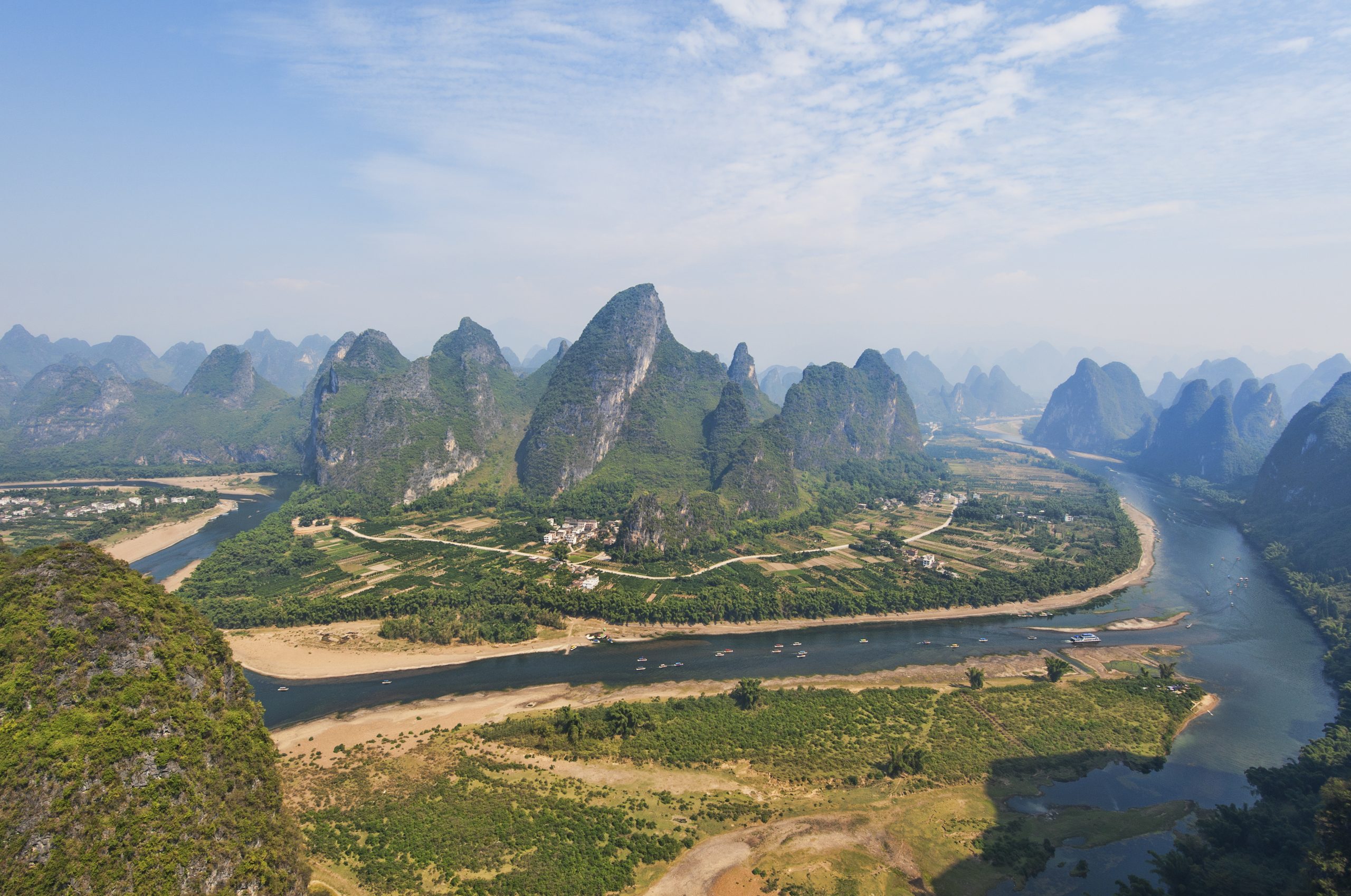
Karst refers to landscapes and hydrologic features created by the dissolving of limestone. Karst can be found anywhere there is limestone and other soluble subterranean substances like salt deposits. Dissolving of limestone creates features like sinkholes, caverns, disappearing streams, and towers.
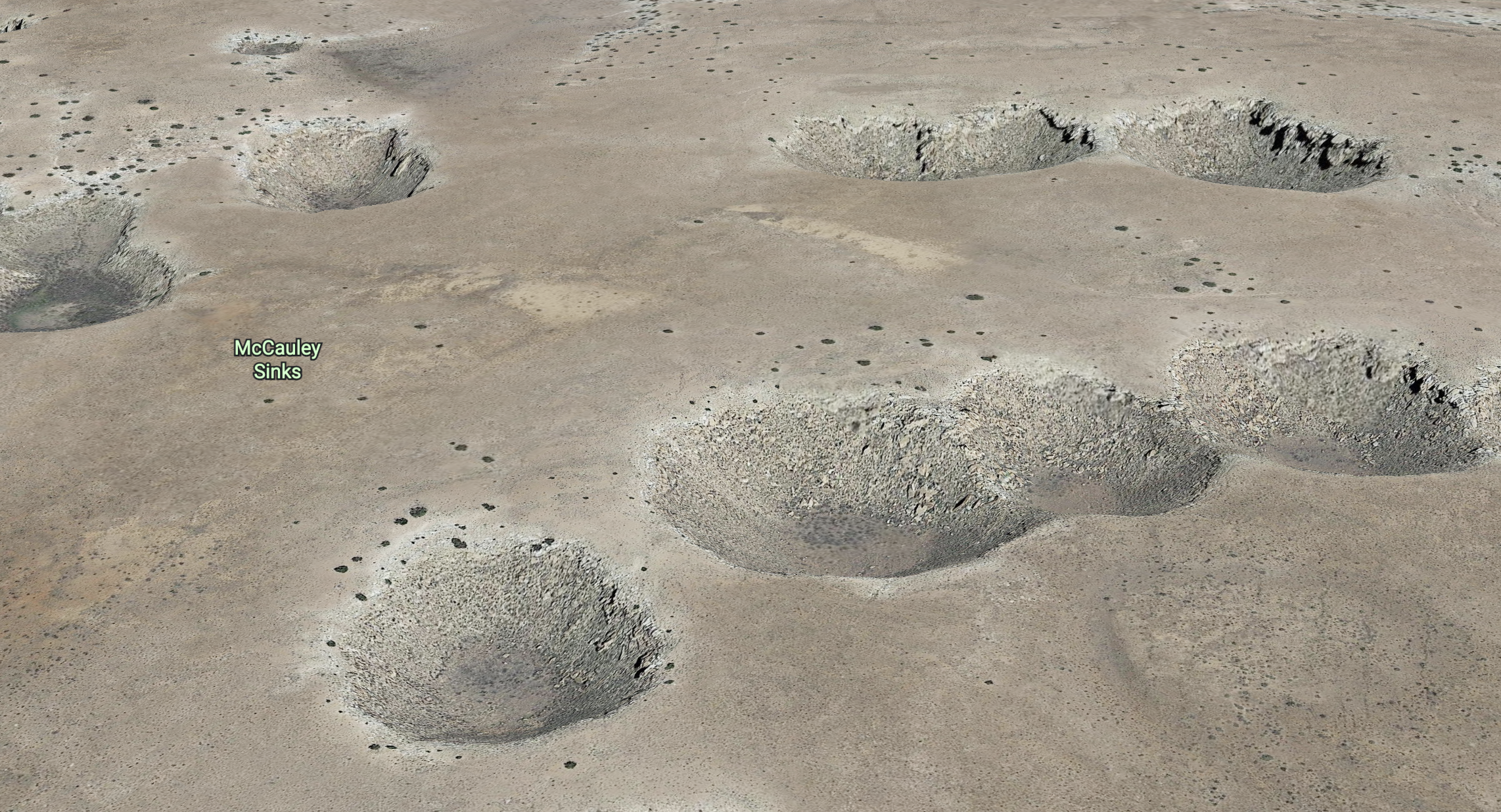
Dissolving of underlying salt deposits has caused sinkholes to form in the Kaibab Limestone on the Colorado Plateau in Arizona.
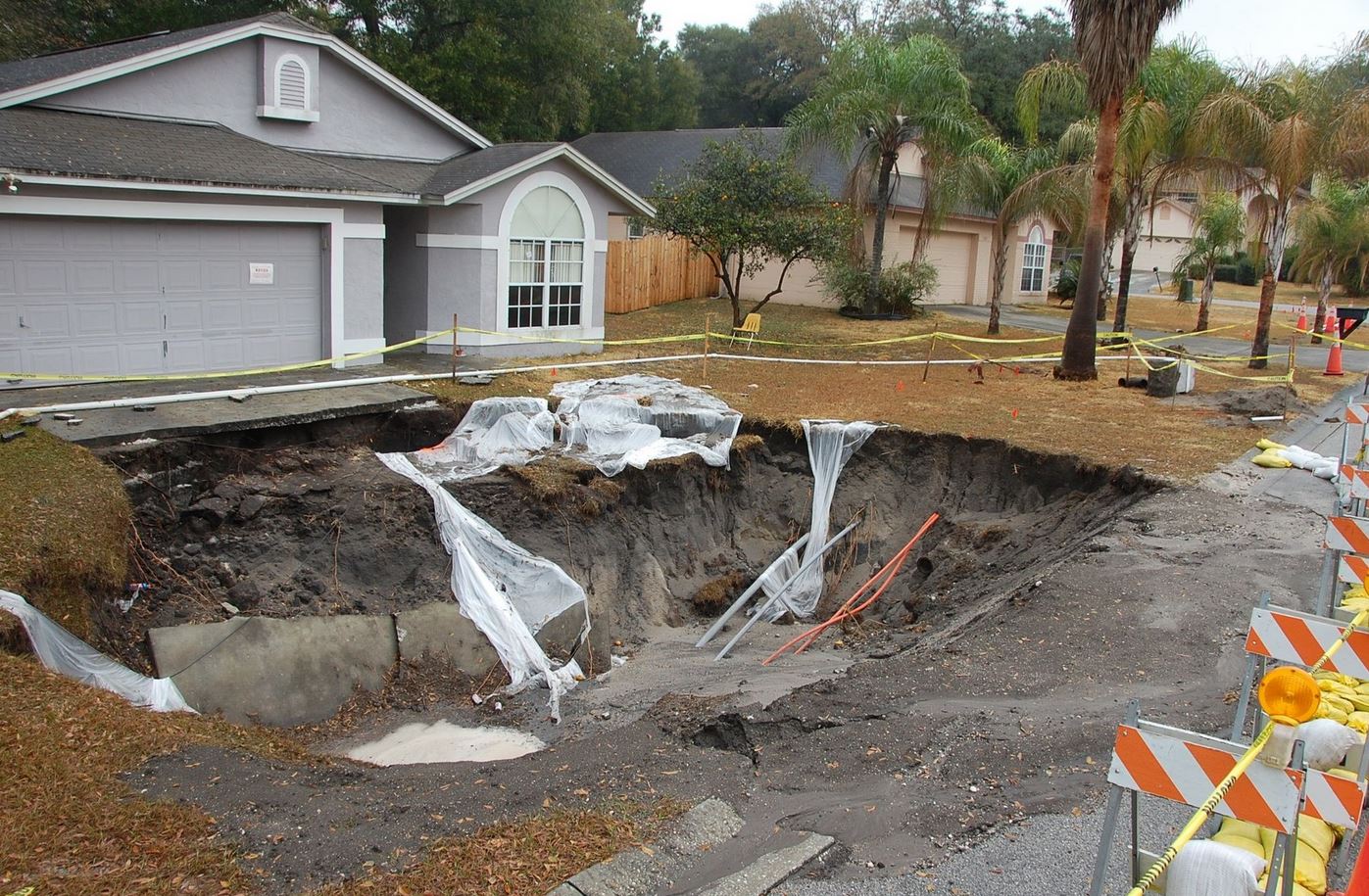
Collapse of the surface into an underground cavern caused this sinkhole in the front yard of a home in Florida.
CO2 in the atmosphere dissolves readily in the water droplets that form clouds from which precipitation comes in the form of rain and snow. This precipitation is slightly acidic with carbonic acid. Karst forms when carbonic acid dissolves calcite (calcium carbonate) in limestone.
H2O + CO2 = H2CO3
Water + Carbon Dioxide Gas equals Carbonic Acid in Water
CaCO3 + H2CO3 = Ca2++ 2HCO3 -1
Solid Calcite + Carbonic Acid in Water Dissolved equals Calcium Ion + Dissolved Bicarbonate Ion
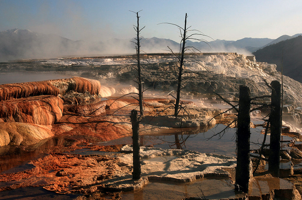
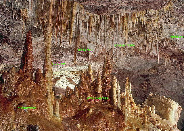
After the slightly acidic water dissolves the calcite, changes in temperature or gas content in the water can cause the water to redeposit the calcite in a different place as tufa (travertine), often deposited by a spring or in a cave. Speleothems are secondary deposits, typically made of travertine, deposited in a cave. Travertine speleothems form by water dripping through cracks and dissolved openings in caves and evaporating, leaving behind the travertine deposits. Speleothems commonly occur in the form of stalactites, when extending from the ceiling, and stalagmites, when standing up from the floor.
Surface water enters the karst system through sinkholes, losing streams, and disappearing streams. Changes in base level can cause rivers running over limestone to dissolve the limestone and sink into the ground. As the water continues to dissolve its way through the limestone, it can leave behind intricate networks of caves and narrow passages. Often dissolution will follow and expand fractures in the limestone. Water exits the karst system as springs and rises. In mountainous terrane, dissolution can extend all the way through the vertical profile of the mountain, with caverns dropping thousands of feet.

Take this quiz to check your comprehension of this section.
If you are using an offline version of this text, access the quiz for section 11.8 via the QR code.
Summary
Water is essential for all living things. It continuously cycles through the atmosphere, over land, and through the ground. In much of the United States and other countries, water is managed through a system of regional laws and regulations and distributed on paper in a system collectively known as “water rights”. Surface water follows a watershed, which is separate from other areas by its divides (highest ridges). Groundwater exists in the pores within rocks and sediment. It moves predominantly due to pressure and gravitational gradients through the rock. Human and natural causes can make water unsuitable for consumption. There are different ways to deal with this contamination. Karst is when limestone is dissolved by water, forming caves and sinkholes.

Take this quiz to check your comprehension of this chapter.
If you are using an offline version of this text, access the quiz for chapter 11 via the QR code.
URLs Linked Within This Chapter
NPR story on Snake Valley: https://www.npr.org/2007/06/12/10953190/las-vegas-water-battle-crops-vs-craps
SNWA History: https://www.snwa.com/about/mission/index.html#:~:text=In%201991%2C%20seven%20local%20water,Big%20Bend%20Water%20District
Dean Baker Story: The Consequences: Transporting Snake Valley water to satisfy a thirsty Las Vegas. [Video: 25:24] https://www.youtube.com/watch?v=eCZ8KLrmUXo
NASA images: https://earthobservatory.nasa.gov/images/8103/mississippi-river-delta
USGS Groundwater Watch: https://groundwaterwatch.usgs.gov/default.asp
USGS tables on contaminants found in groundwater: https://www.usgs.gov/special-topics/water-science-school/science/contamination-groundwater
Text References
- Brush, L.M., Jr, 1961, Drainage basins, channels, and flow characteristics of selected streams in central Pennsylvania: pubs.er.usgs.gov.
- Charlton, R., 2007, Fundamentals of fluvial geomorphology: Taylor & Francis.
- Cirrus Ecological Solutions, 2009, Jordan River TMDL: Utah State Division of Water Quality.
- Earle, S., 2015, Physical geology OER textbook: BC Campus OpenEd.
- EPA, 2009, Water on Tap-What You Need to Know: U.S. Environmental Protection Agency.
- Fagan, B., 2012, Elixir: A history of water and humankind: Bloomsbury Press.
- Fairbridge, R.W., 1968, Yazoo rivers or streams, in Geomorphology: Springer Berlin Heidelberg Encyclopedia of Earth Science, p. 1238–1239.
- Freeze, A.R., and Cherry, J.A., 1979, Groundwater: Prentice Hall.
- Galloway, D., Jones, D.R., and Ingebritsen, S.E., 1999, Land subsidence in the United States: U.S. Geological Survey Circular 1182.
- Galloway, W.E., Whiteaker, T.L., and Ganey-Curry, P., 2011, History of Cenozoic North American drainage basin evolution, sediment yield, and accumulation in the Gulf of Mexico basin: Geosphere, v. 7, no. 4, p. 938–973.
- Gilbert, G.K., 1890, Lake Bonneville: United States Geological Survey, 438 p.
- Gleick, P.H., 1993, Water in Crisis: A Guide to the World’s Fresh Water Resources: Oxford University Press.
- Hadley, G., 1735, Concerning the cause of the general trade-winds: By Geo. Hadley, Esq; FRS: Philosophical Transactions, v. 39, no. 436–444, p. 58–62.
- Halvorson, S.F., and James Steenburgh, W., 1999, Climatology of lake-effect snowstorms of the Great Salt Lake: University of Utah.
- Heath, R.C., 1983, Basic ground-water hydrology: U.S. Geological Survey Water-Supply Paper 2220, 91 p.
- Hobbs, W.H., and Fisk, H.N., 1947, Geological Investigation of the Alluvial Valley of the Lower Mississippi River: JSTOR.
- Knudsen, T., Inkenbrandt, P., Lund, W., Lowe, M., and Bowman, S., 2014, Investigation of land subsidence and earth fissures in Cedar Valley, Iron County, Utah: Utah Geological Survey Special Study 150.
- Lorenz, E.N., 1955, Available potential energy and the maintenance of the general circulation: Tell’Us, v. 7, no. 2, p. 157–167.
- Marston, R.A., Mills, J.D., Wrazien, D.R., Bassett, B., and Splinter, D.K., 2005, Effects of Jackson lake dam on the Snake River and its floodplain, Grand Teton National Park, Wyoming, USA: Geomorphology, v. 71, no. 1–2, p. 79–98.
- Maupin, M.A., Kenny, J.F., Hutson, S.S., Lovelace, J.K., Barber, N.L., and Linsey, K.S., 2014, Estimated use of water in the United States in 2010: US Geological Survey.
- Myers, W.B., and Hamilton, W., 1964, The Hebgen Lake, Montana, earthquake of August 17, 1959: U.S. Geol. Surv. Prof. Pap., v. 435, p. 51.
- Oviatt, C.G., 2015, Chronology of Lake Bonneville, 30,000 to 10,000 yr B.P: Quat. Sci. Rev., v. 110, p. 166–171.
- Powell, J.W., 1879, Report on the lands of the arid region of the United States with a more detailed account of the land of Utah with maps: Monograph.
- Reed, J.C., Love, D., and Pierce, K., 2003, Creation of the Teton landscape: a geologic chronicle of Jackson Hole and the Teton Range: pubs.er.usgs.gov.
- Reese, R.S., 2014, Review of Aquifer Storage and Recovery in the Floridan Aquifer System of Southern Florida.
- Schele, L., Miller, M.E., Kerr, J., Coe, M.D., and Sano, E.J., 1992, The Blood of Kings: Dynasty and Ritual in Maya Art: George Braziller Inc.
- Seaber, P.R., Kapinos, F.P., and Knapp, G.L., 1987, Hydrologic unit maps.
- Solomon, S., 2011, Water: The Epic Struggle for Wealth, Power, and Civilization: Harper Perennial.
- Törnqvist, T.E., Wallace, D.J., Storms, J.E.A., Wallinga, J., Van Dam, R.L., Blaauw, M., Derksen, M.S., Klerks, C.J.W., Meijneken, C., and Snijders, E.M.A., 2008, Mississippi Delta subsidence primarily caused by compaction of Holocene strata: Nat. Geosci., v. 1, no. 3, p. 173–176.
- Turner, R.E., and Rabalais, N.N., 1991, Changes in Mississippi River water quality this century: Bioscience, v. 41, no. 3, p. 140–147.
- United States Geological Survey, 1967, The Amazon: Measuring a Mighty River: United States Geological Survey O-245-247.
- U.S. Environmental Protection Agency, 2014, Cyanobacteria/Cyanotoxins.
- U.S. Geological Survey, 2012, Snowmelt – The Water Cycle, from USGS Water-Science School.
- Utah/Nevada Draft Snake Valley Agreement, 2013.
Figure References
Figure 11.1: Example of a Roman aqueduct in Segovia, Spain. Bernard Gagnon. 2009. CC BY-SA 3.0. https://en.wikipedia.org/wiki/File:Aqueduct_of_Segovia_08.jpg
Figure 11.2: Chac mask in Mexico. Bernard DUPONT. 1995. CC BY-SA 2.0. https://commons.wikimedia.org/wiki/File:Chac_Mask_(21784027699).jpg
Figure 11.3: The water cycle. John Evans and Howard Periman, USGS. 2013. Public domain. https://commons.wikimedia.org/wiki/File:Watercyclesummary.jpg
Figure 11.4: Map view of a drainage basin with main trunk streams and many tributaries with drainage divide in dashed red line. Zimbres. 2005. CC BY-SA 2.5. https://commons.wikimedia.org/wiki/File:Hydrographic_basin.svg
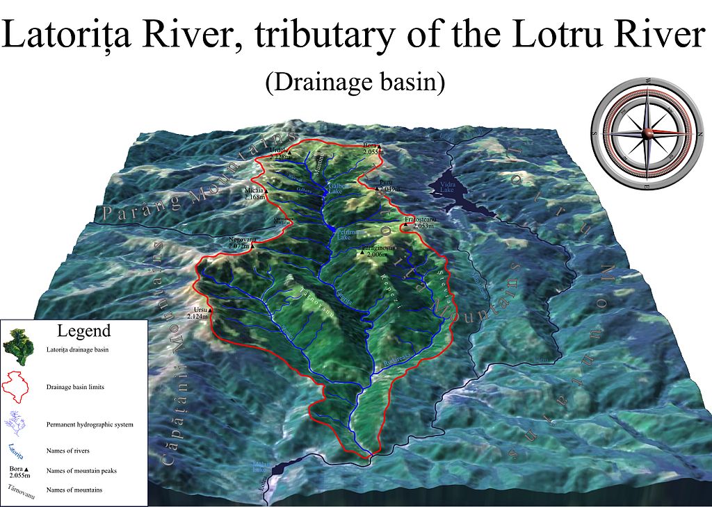
Figure 11.5: Oblique view of the drainage basin and divide of the Latorita River, Romania. Asybaris01. 2011. Public domain. https://commons.wikimedia.org/wiki/File:EN_Bazinul_hidrografic_al_Raului_Latorita,_Romania.jpg
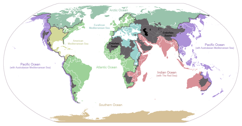
Figure 11.6: Major drainage basins color coded to match the related ocean. Citynoise. 2007. Public domain. https://commons.wikimedia.org/wiki/File:Ocean_drainage.png
Figure 11.7: Agricultural water use in the United States by state. USGS. 2018. Public domain. https://www.usgs.gov/media/images/map-us-state-showing-total-water-withdrawals-2015
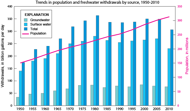
Figure 11.8: Trends in water use by source. USGS. 2018. Public domain. https://www.usgs.gov/media/images/trends-population-and-freshwater-withdrawals-source-1950-2015-0
Figure 11.9: Distribution of precipitation in the United States. United States Department of the Interior. 2006. Public domain. https://commons.wikimedia.org/wiki/File:Average_precipitation_in_the_lower_48_states_of_the_USA.png
Figure 11.10: Thalweg of a river. In a river bend, the fastest moving water is on the outside of the bend, near the cutbank. Steven Earle. 2021. CC BY. Figure 8.1.1 from https://openeducationalberta.ca/practicalgeology/chapter/8-1-stream-erosion-and-deposition/#fig8.1.1
Figure 11.11: Various stream drainage patterns. Kindred Grey. 2022. CC BY-SA 3.0. Includes Rectangular by Zimbres, 2006 (CC BY-SA 2.5, https://commons.wikimedia.org/wiki/File:Rectangular.png). Dendritic by Zimbres, 2006 (CC BY-SA 2.5, https://en.wikipedia.org/wiki/File:Dendritic.png). Trellis drainage pattern by Tshf aee, 2007 (CC BY-SA 3.0, https://en.wikipedia.org/wiki/File:Trellis_drainage_pattern.JPG). Radial by Zimbres, 2006 (CC BY-SA 2.5, https://commons.wikimedia.org/wiki/File:Radial.png). Irregular drainage pattern by Tshf aee, 2007 (CC BY-SA 3.0, https://en.wikipedia.org/wiki/File:Irregular_drainage_pattern.JPG).
Figure 11.12: A stream carries dissolved load, suspended load, and bedload. PSUEnviroDan. 2008. Public domain. https://en.wikipedia.org/wiki/File:Stream_Load.gif
Figure 11.13: Profile of stream channel at bankfull stage, flood stage, and deposition of natural levee. Steven Earle. 2021. CC BY. Figure 8.1.4 from https://openeducationalberta.ca/practicalgeology/chapter/8-1-stream-erosion-and-deposition/#retfig8.1.3
Figure 11.14: Example of a longitudinal profile of a stream; Halfway Creek, Indiana. USGS. 2008. Public domain. https://commons.wikimedia.org/wiki/File:HalfwayCreek_fig02.jpg
Figure 11.15: The braided Waimakariri river in New Zealand. Greg O’Beirne. 2007. CC BY 2.5. https://www.wikiwand.com/simple/Braided_river#Media/File:Waimakariri01_gobeirne.jpg
Figure 11.16: Air photo of the meandering river, Río Cauto, Cuba. Not home~commonswiki. 2007. Public domain. https://commons.wikimedia.org/wiki/File:Rio-cauto-cuba.JPG
Figure 11.17: Point bar and cut bank on the Cirque de la Madeleine in France. Jean-Christophe BENOIST. 2007. CC BY 2.5. https://www.wikiwand.com/en/Bar_(river_morphology)#Media/File:CirqueMadeleine.jpg
Figure 11.18: An entrenched meander on the Colorado River in the eastern entrance to the Grand Canyon. Paul Hermans. 2012. CC BY-SA 3.0. https://commons.wikimedia.org/wiki/File:Horseshoe_Bend_TC_27-09-2012_15-34-14.jpg
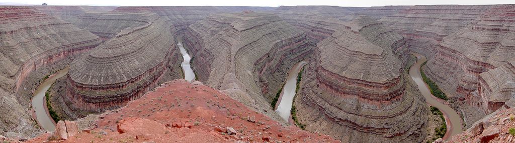
Figure 11.19: Panoramic view of incised meanders of the San Juan River at Gooseneck State Park, Utah. Michael Rissi. 2006. CC BY-SA 3.0. https://commons.wikimedia.org/wiki/File:GooseNeckStateParkPanorama.jpg
Figure 11.20: The Rincon is an abandoned meander loop on the entrenched Colorado River in Lake Powell. NASA’s Earth Observatory. 2012. CC BY 2.0. https://commons.wikimedia.org/wiki/File:Lake_Powell_and_The_Rincon,_Utah_-_NASA_Earth_Observatory.jpg
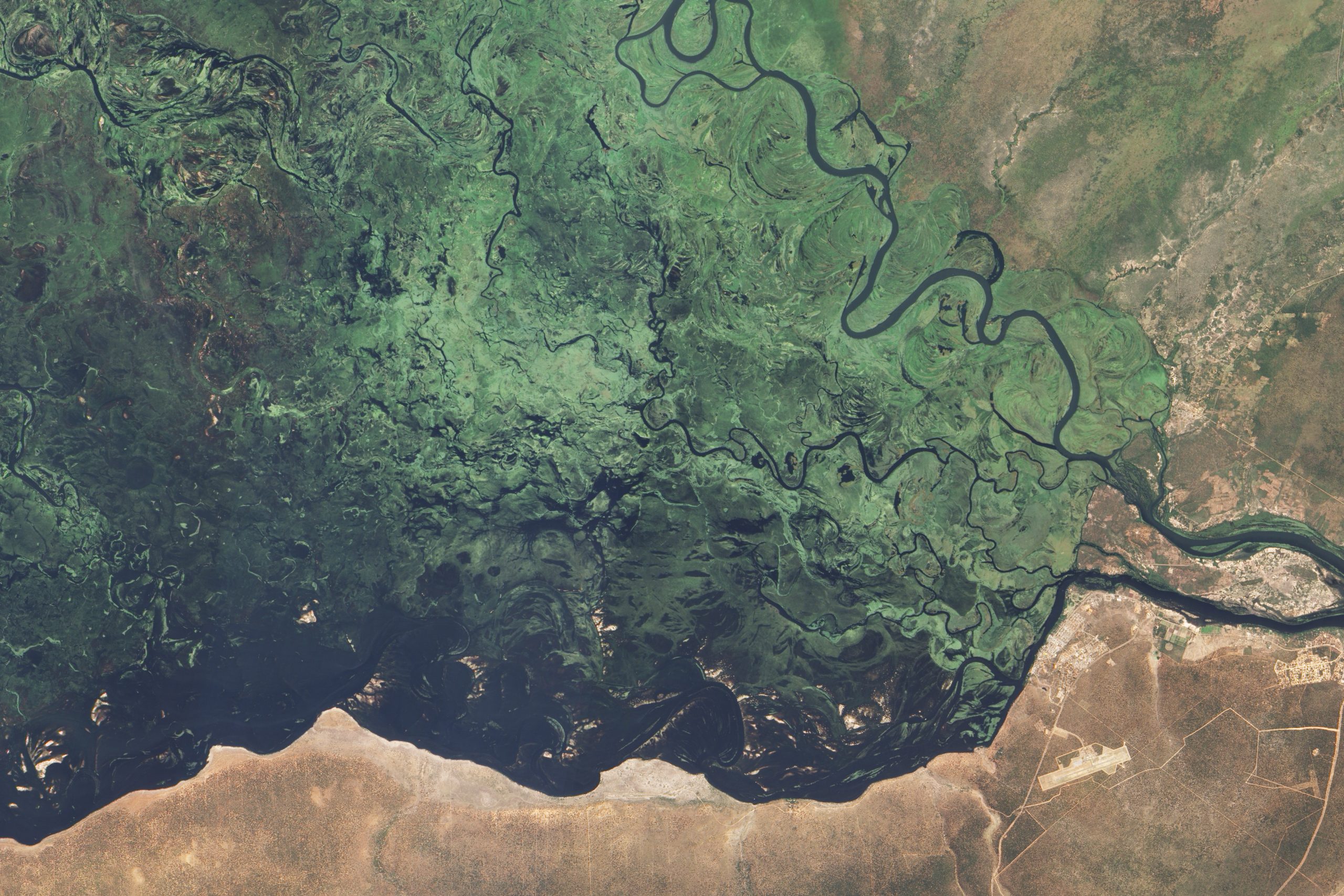
Figure 11.21: Landsat image of Zambezi Flood Plain, Namibia. Jesse Allen and Robert Simmon
via NASA. 2010. Public domain. https://commons.wikimedia.org/wiki/File:Zambezi_Flood_Plain,_Namibia_(EO-1).jpg
Figure 11.22: Meander nearing cutoff on the Nowitna River in Alaska. Oliver Kurmis. 2002. CC BY-SA 2.0 DE. https://www.wikiwand.com/en/Oxbow_lake#Media/File:Nowitna_river.jpg
Figure 11.23: Alluvial fan in Iraq seen by NASA satellite. NASA. 2004. Public domain. https://commons.wikimedia.org/wiki/File:Alluvial_fan_in_Iran.jpg
Figure 11.24: Location of the Mississippi River drainage basin and Mississippi River delta. Shannon1. 2016. CC BY-SA 4.0. https://commons.wikimedia.org/wiki/File:Mississippiriver-new-01.png
Figure 11.25: Delta in Quake Lake Montana. Staplegunther. 2007. CC BY-SA 3.0. https://commons.wikimedia.org/wiki/File:Quakelakemontana.jpg
Figure 11.26: Sundarban Delta in Bangladesh, a tide-dominated delta of the Ganges River. NordNordWest. 2015. CC BY-SA 3.0 DE. https://commons.wikimedia.org/wiki/File:Bangladesh_adm_location_map.svg
Figure 11.27: Nile Delta showing its classic “delta” shape. NASA. 2018. Public domain. https://www.earthdata.nasa.gov/worldview/worldview-image-archive/the-nile-delta-from-space
Figure 11.28: Map of Lake Bonneville, showing the outline of the Bonneville shoreline, the highest level of the lake. Staplini. 2019. CC BY-SA 4.0. https://commons.wikimedia.org/wiki/File:Map_of_Lake_Bonneville.jpg
Figure 11.29: Deltaic deposits of Lake Bonneville near Logan, Utah; wave cut terraces can be seen on the mountain slope. Staplini. 2019. CC BY-SA 4.0. https://commons.wikimedia.org/wiki/File:Image_of_Lake_Bonneville_shorelines.png
Figure 11.30: Terraces along the Snake River, Wyoming. Fredlyfish4. 2008. CC BY-SA 3.0. https://commons.wikimedia.org/wiki/File:Snake_River_Overlook.JPG
Figure 11.31: Zone of saturation. USGS. 2011. Public domain. https://commons.wikimedia.org/wiki/File:Vadose_zone.gif
Figure 11.32: An aquifer cross-section. Hans Hillewaert. 2007. CC BY-SA 3.0. https://commons.wikimedia.org/wiki/File:Aquifer_en.svg
Figure 11.33: Pipe showing apparatus that would demonstrate Darcy’s Law. Vectorised by Sushant savla from the work by Peter Kapitola. 2018. CC BY-SA 2.5. https://en.m.wikipedia.org/wiki/File:Darcy%27s_Law.svg
Figure 11.34: Cones of depression. USGS. 2018. Public domain. https://www.usgs.gov/media/images/cone-depression-pumping-a-well-can-cause-water-level-lowering
Figure 11.35: Different ways an aquifer can be recharged. USGS. Unknown date. Public domain. https://www.usgs.gov/media/images/groundwater-can-be-recharged-naturally-and-artificially
Figure 11.36: Evidence of land subsidence from pumping of groundwater shown by dates on a pole. Dr. Joseph F. Poland via USGS. 1977. Public domain. https://www.usgs.gov/media/images/location-maximum-land-subsidence-us-levels-1925-and-1977
Figure 11.37: Steep karst towers in China left as remnants as limestone is dissolved away by acidic rain and groundwater. chensiyuan. 2011. CC BY-SA 4.0. https://commons.wikimedia.org/wiki/File:1_li_jiang_guilin_yangshuo_2011.jpg
Figure 11.38: Sinkholes of the McCauley Sink in Northern Arizona, produced by collapse of Kaibab Limestone into caverns caused by solution of underlying salt deposits. Google Earth. Image retrieved 2022 by Kindred Grey. Public domain.
Figure 11.39: This sinkhole from collapse of surface into a underground cavern appeared in the front yard of this home in Florida. Ann Tihansky via USGS. 2010. Public domain. https://www.usgs.gov/media/images/sinkholes-west-central-florida-freeze-event-2010-2
Figure 11.40: Mammoth hot springs, Yellowstone National Park. Brocken Inaglory. 2008. CC BY-SA 3.0. https://en.wikipedia.org/wiki/File:Dead_trees_at_Mammoth_Hot_Springs.jpg
Figure 11.41: Varieties of speleothems. Dave Bunnell / Under Earth Images. 2006. CC BY-SA 2.5. https://commons.wikimedia.org/wiki/File:Labeled_speleothems.jpg
Figure 11.42: This stream disappears into a subterranean cavern system to re-emerge a few hundred yards downstream. Martyn Gorman. 2007. CC BY-SA 2.0. https://www.geograph.org.uk/photo/471804
The area within a topographic basin or drainage divide in which water collects.
Pieces of rock that have been weathered and possibly eroded.
Sediment gathering together and collecting, typically in a topographic low point.
A channelled body of water.
Depositional environments that are associated with running water.
A channel that carves into existing bedrock, preserving its original shape and character.
An elevated erosional surface caused by glacial or fluvial action.
A rock or sediment that has good permeability and porosity, and allows water to move easily, making it possible to get water for human use.
A layer that has lower permeability and porosity and does not allow fluid flow as easily.
The depth of the groundwater system below which has pore space 100% filled with water.
The process of cleaning up a polluted site.
Carbonate rocks which dissolve, leaving behind caverns and holes which affect the landscape.
The water part of the Earth, as a solid, liquid, or gas.
A natural substance that is typically solid, has a crystalline structure, and is typically formed by inorganic processes. Minerals are the building blocks of most rocks.
The process of turning sediment into sedimentary rock, including deposition, compaction, and cementation.
A process where an oceanic plate descends bellow a less dense plate, causing the removal of the plate from the surface. Subduction causes the largest earthquakes possible, as the subducting plate can lock as it goes down. Volcanism is also caused as the plate releases volatiles into the mantle, causing melting.
The thin, outer layer of the Earth which makes up the rocky bottom of the ocean basins. Oceanic crust is much thinner (but denser) than continental crust. Oceanic crust is made of rocks similar to basalt and as it cools, becomes more dense.
A solid part of the lithosphere which moves as a unit, i.e. the entire plate generally moves the same direction at the same speed.
The process in which volatiles enter the mantle wedge, and the volatiles lower the melting temperature, causing volcanism.
Middle chemical layer of the Earth, made of mainly iron and magnesium silicates. It is generally denser than the crust (except for older oceanic crust) and less dense than the core.
Components of magma which are dissolved until it reaches the surface, where they expand. Examples include water and carbon dioxide. Volatiles also cause flux melting in the mantle, causing volcanism.
Liquid rock within the Earth.
Place where lava is erupted at the surface.
The gases that are part of the Earth, which are mainly nitrogen and oxygen.
The act of a solid coming out of solution, typically resulting from a drop in temperature or a decrease of the dissolving material.
Water that flows over the surface.
Empty space in a geologic material, either within sediments, or within rocks. Can be filled by air, water, or hydrocarbons.
A combination of evaporation and transpiration from plants, which is a measure of water entering the atmosphere.
Water that works its way down into the subsurface.
A type of non-eroded sediment mixed with organic matter, used by plants. Many essential elements for life, like nitrogen, are delivered to organisms via the soil.
Water that is below the surface.
Area where water infiltrates into the ground and adds to the overall groundwater.
Detached, free-falling rocks from very steep slopes.
A natural stream that flows into a larger river or other body of water.
The end of a river.
An internally draining watershed, whose waters do not flow to the ocean.
Amount of water that leaves a system, such as a river or aquifer.
A stream or river that can be wet or dry depending on the season.
Dry riverbed in an arid region.
Dangerous flooding that occurs in arid regions.
Rocks which allow petroleum resources to collect or move.
A down-warped feature in the crust.
An interconnected set of parts that combine and make up a whole.
Long term averages and variations within the conditions of the atmosphere.
Soil and rock which is below freezing for long periods of time.
Term for the extensional tectonic province that extends from California’s Sierra Nevada Mountains in the west, to Utah’s Wasatch Mountains to the east, to southern Oregon and Idaho to the north, to northern Mexico to the south. Known as a wide rift, each graben (basin) is bounded by horsts (ranges).
A body of ice that moves downhill under its own mass.
A purchase or claim to a legal allotment of a water source, obtained through the state government, such as a spring, stream, well, or lake.
A place where pressurized groundwater flows onto the surface.
Elevation of the mouth of a river.
A federally-supported pollution clean-up effort.
Slope of a stream channel.
The transport and movement of weathered sediments.
The theory that the outer layer of the Earth (the lithosphere) is broken in several plates, and these plates move relative to one another, causing the major topographic features of Earth (e.g. mountains, oceans) and most earthquakes and volcanoes.
Deepest part of a meandering channel.
The measure of the vibrational (kinetic) energy of a substance.
The shape or form of a river and/or tributary drainage system.
A rock layer that has been bent in a ductile way instead of breaking (as with faulting).
Planar feature where two blocks of bedrock move past each other via earthquakes.
Drainage pattern in an area of low topography, dominated by bedding planes, joints, and fracture patterns.
A drainage pattern which forms between ridge lines in deformed (typically sedimentary) rocks.
Discernible layers of rock, typically from a sedimentary rock.
A break within a rock that has no relative movement between the sides. Caused by cooling, pressure release, tectonic forces, etc.
Drainage pattern emanating from a high point.
A common branching style of drainage pattern that resembles the pattern of tree roots.
A chemical or biochemical rock made of mainly calcite.
Drainages that are erratic and disappearing, typically in karst environments.
Deposition that has to do with rivers.
Flat area around a river channel that is filled with water during flooding events.
The source or beginning of a river.
Place where rivers enter a large body of water, forming a triangular shape as the river deposits sediment and switches course.
Illustration of the topography of the base of a stream, showing zones of sediment production, transport, and deposition.
Sediment that large and dense, typically sits on the bottom of stream channels, and is only moved with higher-speed flows.
Bedload sediments that can be carried by higher-velocity flows.
Amount of material dissolved in stream water.
Silt and sand that is lifted from the bed and transported for short distances.
The act of taking a solid and dissolving it into a liquid. This commonly occurs with salts and other minerals in water.
Breaking down of mineral material via chemical methods, like dissolution and oxidation.
Largest amount of flow a river can hold before flooding.
Built-up area around a river channel which can hold river flow within a channel.
Erosional part of a meandering channel.
A qualitative measure of the amount of metamorphism that has occurred or the amount of a resource present in an ore.
A sequence of layers in which the sediment changes linearly in size, either getting coarser or finer.
Channel type with many switching channels, common with large sediment volumes.
Low-gradient channel where rivers sweep across broad flood plains.
Pieces of rock that have been weathered and possibly eroded.
Channels that form straight, typically near the headwaters.
Depositional portion of a meandering channel.
Term for the underlying lithified rocks that make up the geologic record in an area. This term can sometimes refer to only the deeper, crystalline (non-layered) rocks.
Sediment that breaks through a levée and deposits in a floodplain during a flood event
Abandoned meanders that are cut off from the main channel.
Silted-in oxbow which still has a topographic expression.
The part of the coastline which is directly related to water-land interaction, specifically the tidal zone and the range of wave base.
A unit of the geologic time scale; smaller than an era, larger than an epoch. We are currently in the Quaternary period.
The act of the land surface down-warping, typically referred to when discussing sedimentation or with rapid groundwater removal.
Sediment being squeezed together into a coherent mass.
An extensive, distinct, and mapped set of geologic layers.
Made or influenced by humans.
A measure of earthquake strength. Scales include Richter and Moment.
General term for sudden material falling (sliding) down a slope due to gravity.
Movements of water (rising and falling) due to the gravity of the moon and sun. This is most often seen in marine settings.
Lakes that form via increased precipitation with glacial climate shifts.
The ability for a fluid to travel between pores, or, how connected the pores are within a rock or sediment.
Amount of empty space within a rock or sediment, including space between grains, fractures, or voids.
The process in which solids (like minerals) are disassociated and the ionic components are dispersed in a liquid (usually water).
Sediment being "glued" together via mineralization, typically calcite and quartz from groundwater fluids.
A very fine-grained rock with very thin layering (fissile).
The measure of how well a fluid flows through an object.
A dark liquid fossil fuel derived from petroleum.
The resistance of a fluid to flow, where a high value means a fluid which does not like to flow (like toothpaste), and a low value means a fluid which flows easily (like water).
A liquid fossil fuel derived from shallow marine rocks (also known as crude oil).
Place where pores are filled with some water and some air, above the water table.
A solution that has the maximum allowed dissolved component, and is unable to dissolve more.
Forces that cause one substance to stick to another.
Forces that hold a substance together.
The height of the water table, if no confining layers or other hindrances present.
A layer with so little porosity and/or permeability that fluids essentially cannot flow through them and only flow around them.
A layer with lower porosity and/or permeability which allows only minimal and/or slow fluid flow.
A well which allows pressurized water to reach the surface.
A proposed explanation for an observation that can be tested.
An observation which is based on numerical data. These observations are preferred because they can be used in calculations.
An accepted scientific idea that explains a process using the best available information.
Area with a lower water table due to water pumping from a well.
A dry lake bed in a desert valley.
Items that are found within Earth that are valuable and limited. Examples include coal, water, and gold.
When discharge exceeds recharge, and the groundwater is withdrawn at a rate that depletes groundwater storage.
Place where material is extracted from the Earth for human use.
Valuable material in the Earth, typically used for metallic mineral resources.
Pollution that comes from one known source.
Pollution that does not come from one specific, known place, but instead, comes from a wide, broad zone.
Minerals that are bonded with the phosphate anion, PO4+3.
Two or more atoms or ions that are connected chemically.
A chemical sedimentary rock that forms as water evaporates.
The deformation that results from application of a stress.
Toxic waters rich in heavy metals and often of low pH that come from unregulated mining districts.
An acid that forms from carbon dioxide and water. It is a large contributor to chemical weathering.
CaCO3. Pure form is clear, but can take on many different colors with impurities. It is soft, fizzes in acid, and has three cleavages that are not at 90°.
Mineral group in which the carbonate ion, CO3-2, is the building block. This can also refer to the rocks that are made from these minerals, namely limestone and dolomite (dolostone).
Porous variety of carbonate that form in relatively unheated water, sometimes as towers and spires.
Porous, concentric, or layered variety of carbonate that forms with often heated water in springs and/or caves.
A geological province which is added (accreted) to a continental mass via subduction and collision.
