4.3 The Binomial Distribution
We have seen how to deal with general discrete random variables, but there are also special cases of DRVs. If we can identify them, they can provide us some insight and shortcuts. The first of these is the binomial distribution.
The Binomial Setting
There are three characteristics of a binomial experiment:
- There are a fixed number of trials. Think of trials as repetitions of an experiment. The letter n denotes the number of trials.
- There are only two possible outcomes for each trial: success and failure. The letter p denotes the probability of a success on one trial, and q denotes the probability of a failure on one trial. Note that p + q = 1.
- The n trials are independent and are repeated using identical conditions. Because they are independent, the outcome of one trial does not help in predicting the outcome of another trial. Another way of saying this is that, for each individual trial, the probability of a success (p) and probability of a failure (q) remain the same.
Let’s say that the withdrawal rate from an elementary physics course at ABC College is 30% for any given term. This implies that, for any given term, 70% of the students stay in the class for the entire term. A “success” could be defined as an individual who withdrew. In this instance, the random variable X represents the number of students who withdraw from the randomly selected elementary physics class.
Any experiment that has the second and third characteristics listed above and where n = 1 is called a Bernoulli trial (named after Jacob Bernoulli who studied them extensively in the late 1600s). A binomial experiment takes place when the number of successes is counted in one or more Bernoulli trials.
For example, randomly guessing at a true-false statistics question has only two outcomes. If a success is guessing correctly, then a failure is guessing incorrectly. If Joe always guesses correctly on any statistics true-false question with probability p = 0.6, then q = 0.4. This means that, for every true-false statistics question Joe answers, his probability of success (p = 0.6) and his probability of failure (q = 0.4) remain the same. This situation meets the binomial requirements.
In contrast, the following example illustrates a problem that is not binomial, as it violates the condition of independence. ABC College has a student advisory committee made up of ten staff members and six students. The committee wishes to choose a chairperson and a recorder. What is the probability that the chairperson and recorder are both students? The names of all committee members are put into a box, and two names are drawn without replacement. The first name drawn determines the chairperson, and the second name, the recorder. There are two trials. However, the trials are not independent because the outcome of the first trial affects the outcome of the second trial. The probability of a student on the first draw is  . The probability of a student on the second draw is
  when the first draw selects a student. The probability is
  when the first draw selects a staff member. The probability of drawing a student’s name changes for each of the trials and, therefore, violates the condition of independence.
Example
Approximately 70% of statistics students do their homework in time for it to be collected and graded. Each student does homework independently. In a statistics class of 50 students, what is the probability that at least 40 will do their homework on time? Students are selected randomly.
This is a binomial problem because there is only a success or a , there are a fixed number of trials, and the probability of a success is 0.70 for each trial.
Solution
failure
If we are interested in the number of students who do their homework on time, then how do we define X?
Solution
X = the number of statistics students who do their homework on time
What values does x take on?
Solution
0, 1, 2, …, 50
What is a “failure,” in words?
Solution
Failure is defined as a student who does not complete their homework on time.
The probability of a success is p = 0.70. The number of trials is n = 50.
If p + q = 1, then what is q?
Solution
q = 0.30
The words “at least” translate as what kind of inequality for the probability question P(x 40).
Solution
Greater than or equal to (≥)
The probability question is P(x ≥ 40).
Your Turn!
Sixty-five percent of people pass the state driver’s exam on the first try. A group of 50 individuals who have taken the driver’s exam is randomly selected. Can we use the binomial here?
Notation for the Binomial
The outcomes of a binomial experiment fit a binomial probability distribution. The random variable X counts the number of successes obtained in n independent trials.
X ~ B(n, p)
Read this as “X is a random variable with a binomial distribution.” The parameters are n and p (n = number of trials, p = probability of a success on each trial).
Since the binomial counts the number of successes, x, in n trials, the range of values for a binomial random variable could be anything from 0 to n (x = 0, 1, 2, …, n).
Binomial Probability Function
Once we have decided the binomial is applicable for a given situation, we can use the binomial probability function to find the probability of a specific number of successes, P(X = x). The binomial probability mass function (PMF) is made up of two parts.
First, we need to find out how many different ways we can get x successes in n trials. To do this, we can use the choose function, also called the binomial coefficient, written as:
nCx = 
NOTE: The ! mark is the factorial operator.
The next part gives us the probability of a single one of those ways to get x successes in n trials. We can achieve this by using our independent multiplication rule, in which we multiply the probability of success (p) raised to the number of successes (x) by the probability of failure (q = 1 – p) raised to the number of failures (n – x).
pxq(n-x)
Since we know each of these ways are equally likely and how many ways are possible, we can now put the two pieces together. We multiply the probability of one way by how many we have, giving us our overall probability of x successes in n trials.
P(X = x) =  pxq(n-x)
Unfortunately the binomial does not have a nice form of cumulative distribution function (CDF), but it is simply the sum of PDFs up until that point. Consider the following example to demonstrate this point.
Example
It has been stated that about 41% of adult workers have a high school diploma but do not pursue any further education. Twenty adult workers are randomly selected.
Let X represent the number of workers who have a high school diploma but do not pursue any further education.
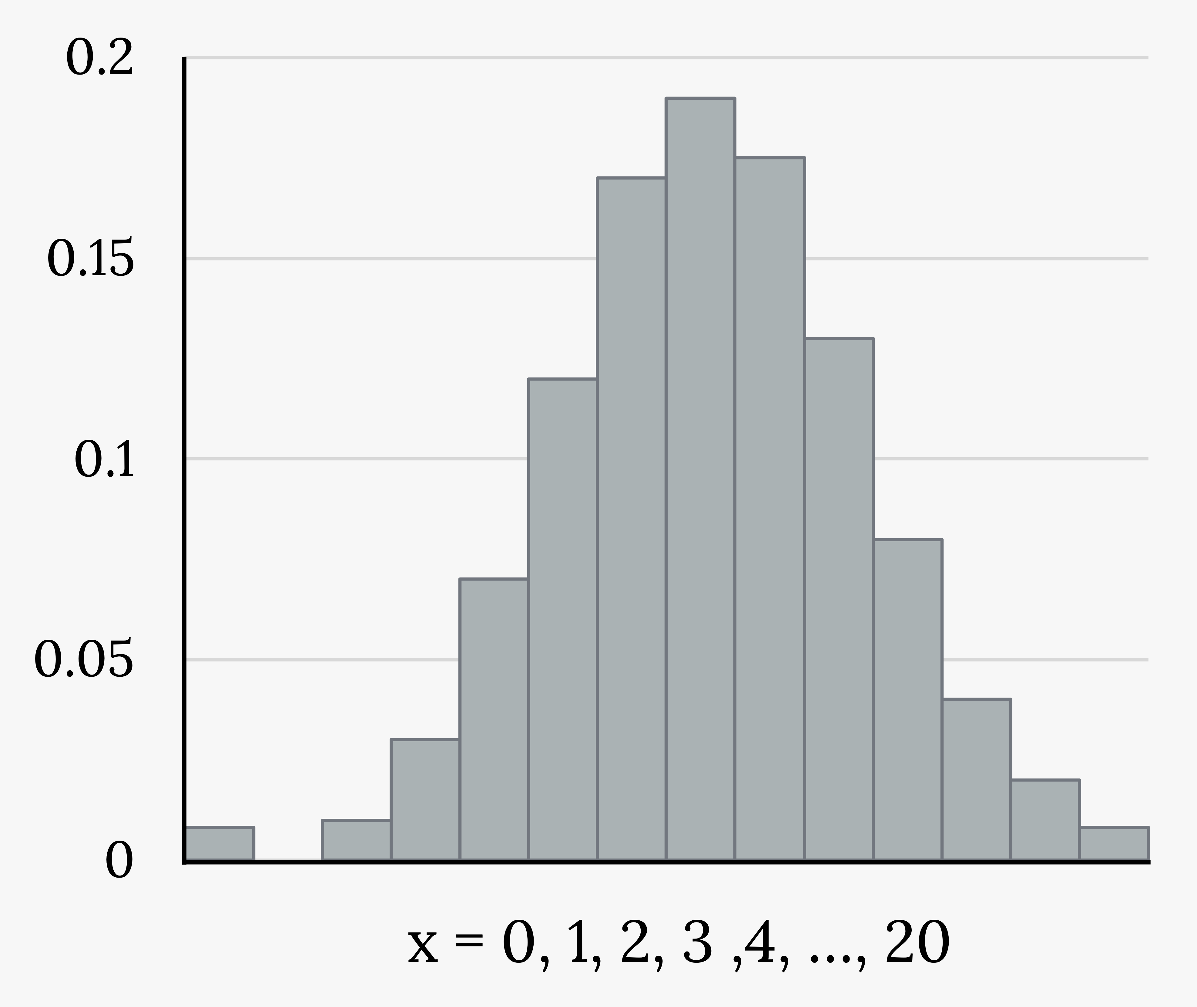
X takes on the values 0, 1, 2, …, 20, where n = 20, p = 0.41, and q = 1 – 0.41 = 0.59.
X ~ B(20, 0.41)
The y-axis contains the probability of x, where X is the number of workers who have only a high school diploma.
The graph of X ~ B(20, 0.41) is as follows:
Find the probability that exactly 12 of them have a high school diploma.
Solution
We can simply plug into the binomial PMF
P(X = x) = pxq(n-x)
for P(X=12) with n=20 and p=0.41,  0.4112(1-0.41)(20-12)
Find the probability that at most 12 of them have a high school diploma but do not pursue any further education. How many adult workers do you expect to have a high school diploma without pursuing any further education?
Solution
If you want to find P(x = 12), use the pdf (binompdf). If you want to find P(x > 12), use 1 – binomcdf(20, 0.41, 12).
The probability that at most 12 workers have a high school diploma but do not pursue any further education is 0.9738.
Your Turn!
About 32% of students participate in a community volunteer program outside of school. If 30 students are selected at random, find:
(a) The probability that exactly 14 of them participate in a community volunteer program outside of school. First, try plugging in to the binomial formula by hand, then check yourself with technology.
(b) The probability that exactly 14 of them participate in a community volunteer program outside of school. Rely on technology for this cumulative probability.
Measures of the Binomial Distribution
The mean, μ, and variance, σ2, for the binomial probability distribution are μ = np and σ2 = npq. The standard deviation, σ, is then σ =  .
.
Example
In the 2013 Jerry’s Artarama art supplies catalog, there are 560 pages. Eight of the pages feature signature artists. Suppose we randomly sample 100 pages. Let X represent the number of pages that feature signature artists.
-
- What values does x take on?
- What is the probability distribution? Find the following probabilities:
- The probability that two pages feature signature artists
- The probability that at most six pages feature signature artists
- The probability that more than three pages feature signature artists
- Using the formulas, calculate the mean and standard deviation.
Solution
1. x = 0, 1, 2, 3, 4, 5, 6, 7, 8
2. X ~ B(100,  )
)
a. P(x = 2) = binompdf(100, , 2) = 0.2466
b. P(x ≤ 6) = binomcdf(100, , 6) = 0.9994
c. P(x > 3) = 1 – P(x ≤ 3) = 1 – binomcdf(100, , 3) = 1 – 0.9443 = 0.0557
3. Mean = np = (100)() = ≈ 1.4286
Standard deviation = =  ≈ 1.1867
Your Turn!
According to a Gallup poll, 60% of American adults prefer saving over spending. Let X represent the number of American adults out of a random sample of 50 who prefer saving to spending.
- What is the probability distribution for X?
- Use your calculator to find the following probabilities:
- The probability that 25 adults in the sample prefer saving over spending
- The probability that at most 20 adults prefer saving
- The probability that more than 30 adults prefer saving
- Using the formulas, calculate the mean and standard deviation of X.
Additional Resources
Figure References
Figure 4.10: Kindred Grey (2020). Workers with diplomas. CC BY-SA 4.0.
Figure Descriptions
Figure 4.10: Histogram showing a binomial probability distribution. It is made up of bars that are fairly normally distributed. The x-axis shows values from zero to 20. The y-axis shows values from zero to 0.2 in increments of 0.05.
A random variable that counts the number of successes in a fixed number (n) of independent Bernoulli trials each with probability of a success (p)
The occurrence of one event has no effect on the probability of the occurrence of another event.
An experiment with the following characteristics:
- There are only two possible outcomes (called “success” and “failure”) for each trial.
- The probability (p) of a success is the same for any trial (so the probability q = 1 − p of a failure is the same for any trial).
A function that gives the probability that a discrete random variable is exactly equal to some value (x)
A function that gives the probability that a random variable takes a value less than or equal to x
