Chapter 3 Extra Practice
3.1 Introduction to Bivariate Data
1. The following figure shows a random sample of 100 hikers and the areas of hiking they prefer.
| Sex | The coastline | Near lakes and streams | One mountain peaks | Total |
|---|---|---|---|---|
| Female | 18 | 16 | ___ | 45 |
| Male | ___ | ___ | 14 | 55 |
| Total | ___ | 41 | ___ | ___ |
Figure 3.26
- Complete the table.
- Are the events “being female” and “preferring the coastline” independent events?Let F = being female, and let C = preferring the coastline.
- Find P(F AND C).
- Find P(F)P(C)
Are these two numbers the same? If they are, then F and C are independent. If they are not, then F and C are not independent.
-
Find the probability that a person is male, given that the person prefers hiking near lakes and streams. Let M = being male, and let L = preferring hiking near lakes and streams.
- What word tells you this is a conditional?
- Fill in the blanks, and calculate the probability: P( | ) = .
- Is the sample space for this problem all 100 hikers? If not, what is it?
-
Find the probability that a person is female or prefers hiking on mountain peaks. Let F = being female, and let P = preferring mountain peaks.
- Find P(F).
- Find P(P).
- Find P(F AND P).
- Find P(F OR P).
2. The figure below shows a random sample of 200 cyclists and the routes they prefer. Let M = males and H = hilly path.
| Gender | Lake path | Hilly path | Wooded path | Total |
|---|---|---|---|---|
| Female | 45 | 38 | 27 | 110 |
| Male | 26 | 52 | 12 | 90 |
| Total | 71 | 90 | 39 | 200 |
Figure 3.27
- Out of the males, what is the probability that the cyclist prefers a hilly path?
- Are the events “being male” and “preferring the hilly path” independent events?
3. Muddy Mouse lives in a cage with three doors. If Muddy goes out the first door, the probability that he gets caught by Alissa the Cat is  and the probability he is not caught is
  . If he goes out the second door, the probability he gets caught by Alissa is
  and the probability he is not caught is
  . The probability that Alissa catches Muddy coming out of the third door is
  , and the probability she does not catch Muddy is . It is equally likely that Muddy will choose any of the three doors, so the probability of choosing each door is
  .
.
| Caught or not | Door 1 | Door 2 | Door 3 | Total |
|---|---|---|---|---|
| Caught |  |
 |
 |
|
| Not caught |  |
 |
|
|
| Total | 1 |
Figure 3.28
- The first entry
 is P(Door 1 AND Caught)
 - The entry
 is P(Door 1 AND Not Caught)
Verify the remaining entries.
- Complete the probability contingency table. Calculate the entries for the totals. Verify that the lower-right corner entry is 1.
- What is the probability that Alissa does not catch Muddy?
- What is the probability that Muddy chooses Door 1 OR Door 2, given that Muddy is caught by Alissa?
4. The figure below relates the weights and heights of a group of individuals participating in an observational study.
| Weight/height | Tall | Medium | Short | Total |
|---|---|---|---|---|
| Obsese | 18 | 28 | 14 | |
| Normal | 20 | 51 | 28 | |
| Underweight | 12 | 25 | 9 | |
| Total |
Figure 3.29
- Find the total for each row and column.
- Find the probability that a randomly chosen individual from this group is Tall.
- Find the probability that a randomly chosen individual from this group is Obese and Tall.
- Find the probability that a randomly chosen individual from this group is Tall, given that the individual is Obese.
- Find the probability that a randomly chosen individual from this group is Obese, given that the individual is Tall.
- Find the probability a randomly chosen individual from this group is Tall and Underweight.
- Are the events Obese and Tall independent?
5. There are several tools you can use to help organize and sort data when calculating probabilities. Contingency tables help display data and are particularly useful when calculating probabilities that have multiple dependent variables.
Use the following information to answer the next four exercises. The figure below shows a random sample of musicians and how they learned to play their instruments.
| Gender | Self-taught | Studied in school | Private instruction | Total |
|---|---|---|---|---|
| Female | 12 | 38 | 22 | 72 |
| Male | 19 | 24 | 15 | 58 |
| Total | 31 | 62 | 37 | 130 |
Figure 3.30
- Find P(musician is a female).
- Find P(musician is a male AND had private instruction).
- Find P(musician is a female OR is self-taught).
- Are the events “being a female musician” and “learning music in school” mutually exclusive events?
6. An article in the New England Journal of Medicine reported about a study of smokers in California and Hawaii. In one part of the report, the self-reported ethnicity and smoking levels per day were given. Of the people smoking at most ten cigarettes per day, there were 9,886 African Americans, 2,745 Native Hawaiians, 12,831 Latinos, 8,378 Japanese Americans, and 7,650 Whites. Of the people smoking 11 to 20 cigarettes per day, there were 6,514 African Americans, 3,062 Native Hawaiians, 4,932 Latinos, 10,680 Japanese Americans, and 9,877 Whites. Of the people smoking 21 to 30 cigarettes per day, there were 1,671 African Americans, 1,419 Native Hawaiians, 1,406 Latinos, 4,715 Japanese Americans, and 6,062 Whites. Of the people smoking at least 31 cigarettes per day, there were 759 African Americans, 788 Native Hawaiians, 800 Latinos, 2,305 Japanese Americans, and 3,970 Whites.[1]
Complete the table using the data provided. Suppose that one person from the study is randomly selected. Find the probability that person smoked 11 to 20 cigarettes per day.
| Smoking level | African American | Native Hawaiian | Latino | Japanese Americans | White | Total |
|---|---|---|---|---|---|---|
| 1-10 | ||||||
| 11-20 | ||||||
| 21-30 | ||||||
| 31+ | ||||||
| Total |
Figure 3.31
- Suppose that one person from the study is randomly selected. Find the probability that person smoked 11 to 20 cigarettes per day.
- Find the probability that the person was Latino.
- In words, explain what it means to pick one person from the study who is “Japanese American AND smokes 21 to 30 cigarettes per day.” Then find the probability.
- In words, explain what it means to pick one person from the study who is “Japanese American OR smokes 21 to 30 cigarettes per day.” Then find the probability.
- In words, explain what it means to pick one person from the study who is “Japanese American GIVEN that person smokes 21 to 30 cigarettes per day.” Then find the probability.
- Prove that smoking level and ethnicity are dependent events.
7. The figure below contains the number of crimes per 100,000 inhabitants from 2008 to 2011 in the US.[2]
| Year | Robbery | Burglary | Rape | Vehicle | Total |
|---|---|---|---|---|---|
| 2008 | 145.7 | 732.1 | 29.7 | 314.7 | |
| 2009 | 133.1 | 717.7 | 29.1 | 259.2 | |
| 2010 | 119.3 | 701 | 27.7 | 239.1 | |
| 2011 | 113.7 | 702.2 | 26.8 | 229.6 | |
| Total |
Figure 3.32
Total each column and each row. Total data = 4,520.7.
- Find P (2009 AND Robbery).
- Find P (2010 AND Burglary).
- Find P (2010 OR Burglary).
- Find P (2011|Rape).
- Find P (Vehicle|2008).
8. In an urn, there are 11 balls. Three balls are red (R), and eight balls are blue (B). Draw two balls, one at a time, with replacement. “With replacement” means that you put the first ball back in the urn before you select the second ball. The tree diagram using frequencies that show all the possible outcomes follows is seen in the figure below.
Total = 64 + 24 + 24 + 9 = 121
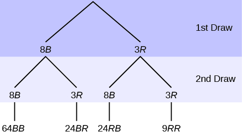
The first set of branches represents the first draw. The second set of branches represents the second draw. Each of the outcomes is distinct. In fact, we can list each red ball as R1, R2, and R3 and each blue ball as B1, B2, B3, B4, B5, B6, B7, and B8. Then the nine RR outcomes can be written as:
R1R1R1R2R1R3R2R1R2R2R2R3R3R1R3R2R3R3
The other outcomes are similar.
There are a total of 11 balls in the urn. Draw two balls, one at a time, with replacement. There are 11(11) = 121 outcomes, the size of the sample space.
- List the 24 BR outcomes: B1R1, B1R2, B1R3, …
- Using the tree diagram, calculate P(RR).
- Using the tree diagram, calculate P(RB OR BR).
- Using the tree diagram, calculate P(R on first draw AND B on second draw).
- Using the tree diagram, calculate P(R on second draw, GIVEN B on first draw).
- Using the tree diagram, calculate P(BB).
- Using the tree diagram, calculate P(B on the second draw, given R on the first draw).
9. An urn contains three red marbles and eight blue marbles. Draw two marbles, one at a time, from the urn, this time without replacement. “Without replacement” means that you do not put the first ball back before you select the second marble. Figure 3.34 shows a tree diagram for this situation. The branches are labeled with probabilities instead of frequencies. The numbers at the ends of the branches are calculated by multiplying the numbers on the two corresponding branches, for example:


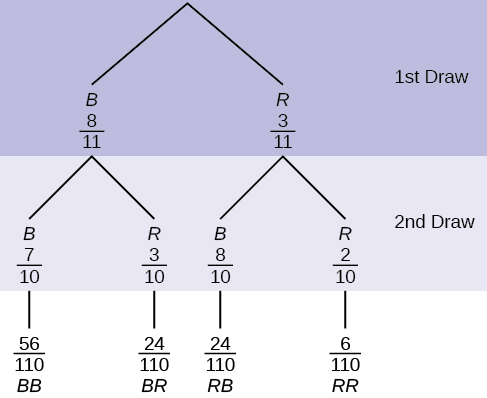
NOTE: If you draw a red on the first draw from the three red possibilities, there are two red marbles left to draw on the second draw. You do not put back or replace the first marble after you have drawn it. You draw without replacement, meaning there are ten marbles left in the urn on the second draw.
Calculate the following probabilities using the tree diagram.
- P(RR)
- P(RB OR BR) =
 + ( )( )=
- P(R on second draw|B on first draw)
- P(R on first draw AND B on second draw) = P(RB) = ( )( ) =

- P(BB)
- P(B on second draw|R on first draw)
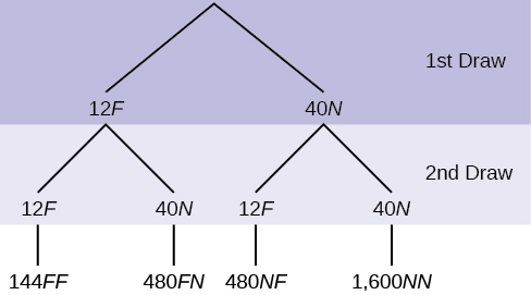
10. In a standard deck, there are 52 cards. 12 cards are face cards (event F), and 40 cards are not face cards (event N). Draw two cards, one at a time, with replacement. All possible outcomes are shown in the tree diagram as frequencies. Using the tree diagram, calculate P(FF).
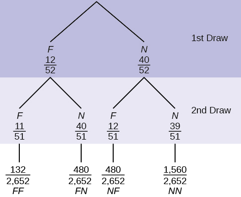
11. In a standard deck, there are 52 cards. Twelve cards are face cards (F), and 40 cards are not face cards (N). Draw two cards, one at a time, without replacement. The tree diagram below is labeled with all possible probabilities.
- Find P(FN OR NF).
- Find P(N|F).
- Find P(at most one face card).
Hint: “At most one face card” means zero or one face card. - Find P(at least one face card).
Hint: “At least one face card” means one or two face cards.
12. A litter of kittens available for adoption at the Humane Society has four tabby kittens and five black kittens. A family comes in and randomly selects two kittens (without replacement) for adoption.
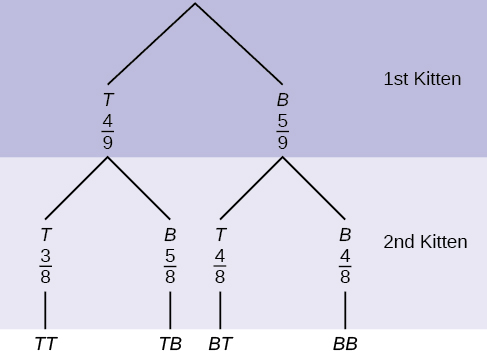
- What is the probability that both kittens are tabby?
a.
b.
c.
d.
2. What is the probability that one kitten of each coloring is selected?
a.
b.
c.
d.
3. What is the probability that a tabby is chosen as the second kitten when a black kitten was chosen as the first?
4. What is the probability of choosing two kittens of the same color?
13. Suppose there are four red balls and three yellow balls in a box. Two balls are drawn from the box without replacement. What is the probability that one ball of each coloring is selected?
14. Flip two fair coins. Let A = tails on the first coin and B = tails on the second coin. Then, A = {TT, TH} and B = {TT, HT}. Therefore:
- A AND B = {TT}
- A OR B = {TH, TT, HT}
The sample space when you flip two fair coins is X = {HH, HT, TH, TT}. The outcome HH is in NEITHER A NOR B. Draw a Venn diagram.
15. Roll a fair, six-sided die. Let A = a prime number of dots being rolled. Let B = an odd number of dots being rolled. If A = {2, 3, 5} and B = {1, 3, 5}, then:
- A AND B = {3, 5}
- A OR B = {1, 2, 3, 5}
The sample space for rolling a fair die is S = {1, 2, 3, 4, 5, 6}. Draw a Venn diagram representing this situation.
16. Suppose an experiment has outcomes black, white, red, orange, yellow, green, blue, and purple, where each outcome has an equal chance of occurring. Let event C = {green, blue, purple} and event P = {red, yellow, blue}. Then C AND P = {blue} and C OR P = {green, blue, purple, red, yellow}. Draw a Venn diagram representing this situation.
17. Fifty percent of the workers at a factory work a second job, 25% have a spouse who also works, and 5% work a second job and have a spouse who also works. Draw a Venn diagram showing the relationships. Let W = working a second job and S = spouse also working.
18. A person with type O blood and a negative Rh factor (Rh-) can donate blood to any person with any blood type. Four percent of African Americans have type O blood and a negative Rh factor, 5−10% of African Americans have the Rh- factor, and 51% have type O blood.[3] [4]
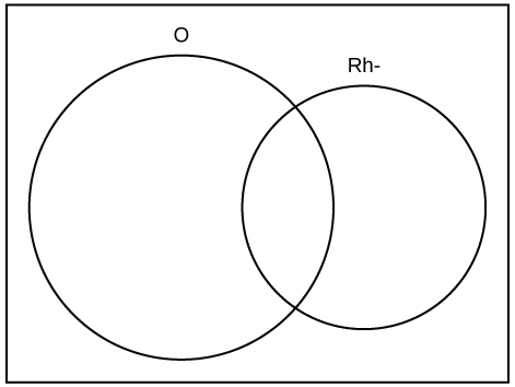
The “O” circle represents the African Americans with type O blood. The “Rh-” oval represents the African Americans with the Rh- factor.
We will take the average of 5% and 10%, using 7.5% as the percent of African Americans who have the Rh- factor. Let O = African American with type O blood and R = African American with Rh- factor.
- Find P(O).
- Find P(R).
- Find P(O AND R).
- Find P(O OR R).
- In a complete sentence, describe the overlapping area of the Venn diagram.
- In a complete sentence, describe the area of the Venn diagram in the rectangle but outside both the circle and the oval.
19. In a bookstore, the probability that the customer buys a novel is 0.6, and the probability that the customer buys a non-fiction book is 0.4. Suppose that the probability that the customer buys both is 0.2.
- Draw a Venn diagram representing the situation.
- Find the probability that the customer buys either a novel or a non-fiction book.
- In the Venn diagram, describe the overlapping area using a complete sentence.
- Suppose that some customers buy only compact discs. Draw an oval in your Venn diagram representing this event.
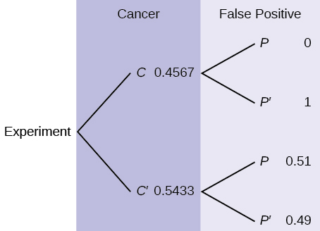
20. The probability that a man develops some form of cancer in his lifetime is 0.4567. The probability that a man has at least one false positive test result (meaning the test comes back for cancer when the man does not have it) is 0.51.[5] Let: C = a man developing cancer in his lifetime and P = man having at least one false positive. Construct a tree diagram of the situation.
21. This tree diagram shows the tossing of an unfair coin followed by drawing one bead from a cup containing three red (R), four yellow (Y), and five blue (B) beads. For the coin, P(H) =  and P(T) = , where H is heads and T is tails.
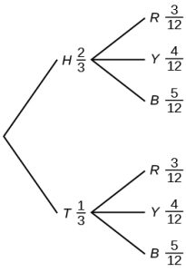
Find P(tossing a head on the coin AND a red bead).


Find P(blue bead).


22. A box of cookies contains three chocolate and seven butter cookies. Miguel randomly selects a cookie and eats it. Then he randomly selects another cookie and eats it.
- Draw the tree that represents the possibilities for the cookie selections. Write the probabilities along each branch of the tree.
- Are the probabilities for the flavor of the second cookie that Miguel selects independent of his first selection? Explain.
- For each complete path through the tree, write the event it represents and find the probabilities.
- Let S be the event that both cookies selected were the same flavor. Find P(S).
- Let T be the event that the cookies selected were different flavors. Find P(T) by two different methods, using the complement rule and using the branches of the tree. Your answers should be the same with both methods.
- Let U be the event that the second cookie selected is a butter cookie. Find P(U).
23. Suppose that you have eight cards. Five are green, and three are yellow. The cards are well shuffled.
Suppose that you randomly draw two cards, one at a time, with replacement. Let G1 = first card is green and G2 = second card is green.
- Draw a tree diagram of the situation.
- Find P(G1 AND G2).
- Find P(at least one green).
- Find P(G2|G1).
- Are G2 and G1 independent events? Explain why or why not.
Suppose that you randomly draw two cards, one at a time, without replacement. Let G1 = first card is green and G2 = second card is green.
- Draw a tree diagram of the situation.
- Find P(G1 AND G2).
- Find P(at least one green).
- Find P(G2|G1).
- Are G2 and G1 independent events? Explain why or why not.
24. The percent of licensed US drivers (from a recent year) that are female is 48.60. Of the females, 5.03% are age 19 and under; 81.36% are age 20–64; and 13.61% are age 65 or over. Of the licensed US male drivers, 5.04% are age 19 and under; 81.43% are age 20–64; and 13.53% are age 65 or over.[6]
Complete the following:
- Construct a table or a tree diagram of the situation.
- Find P(driver is female).
- Find P(driver is age 65 or over|driver is female).
- Find P(driver is age 65 or over AND female).
- In words, explain the difference between the probabilities in part (c) and part (d).
- Find P(driver is age 65 or over).
- Are being age 65 or over and being female mutually exclusive events? How do you know?
Suppose that 10,000 US licensed drivers are randomly selected.
- How many would you expect to be male?
- Using the table or tree diagram, construct a contingency table of gender versus age group.
- Using the contingency table, find the probability that a driver randomly selected from the 20–64 age group is female.
25. Approximately 86.5% of Americans commute to work by car, truck, or van. Out of that group, 84.6% drive alone and 15.4% drive in a carpool. Approximately 3.9% walk to work, and approximately 5.3% take public transportation.[7]
- Construct a table or a tree diagram of the situation. Include a branch for all other modes of transportation to work.
- Assuming that the walkers walk alone, what percent of all commuters travel alone to work?
- Suppose that 1,000 workers are randomly selected. How many would you expect to travel alone to work?
- Suppose that 1,000 workers are randomly selected. How many would you expect to drive in a carpool?
26. When the Euro coin was introduced in 2002, two math professors had their statistics students test whether the Belgian one Euro coin was a fair coin. They spun the coin rather than tossing it and found that 140 of 250 spins showed a head (event H), while 110 showed a tail (event T). On that basis, they claimed that it is not a fair coin.
- Based on the given data, find P(H) and P(T).
- Use a tree to find the probabilities of each possible outcome for the experiment of tossing the coin twice.
- Use the tree to find the probability of obtaining exactly one head in two tosses of the coin.
- Use the tree to find the probability of obtaining at least one head.
27. The following are real data from Santa Clara County, CA. At a certain point in time, there had been a total of 3,059 documented cases of AIDS in the county. They were grouped into the following categories:[8]
| Homosexual/bisexual | IV drug user* | Heterosexual contact | Other | Total | |
|---|---|---|---|---|---|
| Female | 0 | 70 | 136 | 49 | |
| Male | 2,146 | 463 | 60 | 135 | |
| Total | |||||
| *includes homosexual/bisexual IV drug users |
Figure 3.41
Suppose a person with AIDS in Santa Clara County is randomly selected.
- Find P(person is female).
- Find P(person has a risk factor heterosexual contact).
- Find P(person is female OR has a risk factor of IV drug user).
- Find P(person is female AND has a risk factor of homosexual/bisexual).
- Find P(person is male AND has a risk factor of IV drug user).
- Find P(person is female, GIVEN person got the disease from heterosexual contact).
- Construct a Venn diagram. Make one group females and the other group heterosexual contact.
The completed contingency table is as follows:
| Homosexual/bisexual | IV drug user* | Heterosexual contact | Other | Total | |
|---|---|---|---|---|---|
| Female | 0 | 70 | 136 | 49 | 255 |
| Male | 2,146 | 463 | 60 | 135 | 2,804 |
| Total | 2,146 | 533 | 196 | 184 | 3,059 |
| *includes homosexual/bisexual IV drug users |
Figure 3.42
Answer these questions using probability rules. Do NOT use the contingency table. Three thousand fifty-nine cases of AIDS had been reported in Santa Clara County, CA, through a certain date. Those cases will be our population. Of those cases, 6.4% obtained the disease through heterosexual contact and 7.4% are female. Out of the females with the disease, 53.3% got the disease from heterosexual contact.
- Find P(person is female).
- Find P(person obtained the disease through heterosexual contact).
- Find P(person is female, GIVEN person got the disease from heterosexual contact).
- Construct a Venn diagram representing this situation. Make one group females and the other group heterosexual contact. Fill in all values as probabilities.
28. The table shows the political party affiliation of each of 67 members of the US Senate in June 2012 and when they are up for reelection.[9]
| Up for reelection | Democratic party | Republican party | Other | Total |
|---|---|---|---|---|
| November 2014 | 20 | 13 | 0 | |
| November 2016 | 10 | 24 | 0 | |
| Total |
Figure 3.43
- What is the probability that a randomly selected senator has an “Other” affiliation?
- What is the probability that a randomly selected senator is up for reelection in November 2016?
- What is the probability that a randomly selected senator is a Democrat and up for reelection in November 2016?
- What is the probability that a randomly selected senator is a Republican or is up for reelection in November 2014?
- Suppose that a member of the US Senate is randomly selected. Given that the randomly selected senator is up for reelection in November 2016, what is the probability that this senator is a Democrat?
- Suppose that a member of the US Senate is randomly selected. What is the probability that the senator is up for reelection in November 2014, knowing that this senator is a Republican?
- The events “Republican” and “Up for reelection in 2016” are .
- mutually exclusive
- independent
- both mutually exclusive and independent
- neither mutually exclusive nor independent
- The events “Other” and “Up for reelection in November 2016” are .
- mutually exclusive
- independent
- both mutually exclusive and independent
- neither mutually exclusive nor independent
29. The figure below gives the number of suicides estimated in the US for a recent year by age, race (Black or White), and sex. We are interested in possible relationships between age, race, and sex. We will let suicide victims be our population.
| Race and sex | 1-14 | 15-24 | 25-64 | Over 64 | Total |
|---|---|---|---|---|---|
| White, male | 210 | 3,360 | 13,610 | 22,050 | |
| White, female | 80 | 580 | 3,380 | 4,930 | |
| Black, male | 10 | 460 | 1,060 | 1,670 | |
| Black, female | 0 | 40 | 270 | 330 | |
| All others | |||||
| Total | 310 | 4,650 | 18,780 | 29,760 |
Figure 3.44
Do not include “all others.”
- Fill in the column for the suicides for individuals over age 64.
- Fill in the row for all other races.
- Find the probability that a randomly selected individual was a White male.
- Find the probability that a randomly selected individual was a Black female.
- Find the probability that a randomly selected individual was Black.
- Find the probability that a randomly selected individual was a Black or White male. Do not include “all others.”
- Out of the individuals over age 64, find the probability that a randomly selected individual was a Black or White male. Do not include “all others.”
30. The table of data obtained from the website Baseball Almanac shows hit information for four well-known baseball players. Suppose that one hit from the table is randomly selected.[10]
| Name | Single | Double | Triple | Home run | Total hits |
|---|---|---|---|---|---|
| Babe Ruth | 1,517 | 506 | 136 | 714 | 2,873 |
| Jackie Robinson | 1,054 | 273 | 54 | 137 | 1,518 |
| Ty Cobb | 3,603 | 174 | 295 | 114 | 4,189 |
| Hank Aaron | 2,294 | 624 | 98 | 755 | 3,771 |
| Total | 8,471 | 1,577 | 583 | 1,720 | 12,351 |
Figure 3.45
Find P(hit was made by Babe Ruth).


Find P(hit was made by Ty Cobb|hit was a home run).


31. The figure below identifies a group of children by one of four hair colors and by type of hair.
| Hair type | Brown | Blond | Black | Red | Total |
|---|---|---|---|---|---|
| Wavy | 20 | 15 | 3 | 43 | |
| Straight | 80 | 15 | 12 | ||
| Total | 20 | 215 |
Figure 3.46
- Complete the table.
- What is the probability that a randomly selected child will have wavy hair?
- What is the probability that a randomly selected child will have either brown or blond hair?
- What is the probability that a randomly selected child will have wavy brown hair?
- What is the probability that a randomly selected child will have red hair, given that he or she has straight hair?
- If B is the event of a child having brown hair, find the probability of the complement of B.
- In words, what does the complement of B represent?
32. In a previous year, the weights of the members of the San Francisco 49ers and the Dallas Cowboys were published in the San Jose Mercury News. The factual data were compiled into the following table.[11]
| Shirt number | ≤ 210 | 211–250 | 251–290 | > 290 |
|---|---|---|---|---|
| 1-33 | 21 | 5 | 0 | 0 |
| 34-66 | 6 | 18 | 7 | 4 |
| 66-99 | 6 | 12 | 22 | 5 |
Figure 3.47
For the following, suppose that you randomly select one player from the 49ers or Cowboys.
- Find the probability that his shirt number is from 1 to 33.
- Find the probability that he weighs at most 210 pounds.
- Find the probability that his shirt number is from 1 to 33 AND he weighs at most 210 pounds.
- Find the probability that his shirt number is from 1 to 33 OR he weighs at most 210 pounds.
- Find the probability that his shirt number is from 1 to 33, GIVEN that he weighs at most 210 pounds.
3.2 Visualizing Bivariate Quantitative Data
1. The Gross Domestic Product Purchasing Power Parity (GDP PPP) is an indication of a country’s currency value compared to another country. The figure below shows the GDP PPP of Cuba as compared to US dollars. Construct a scatter plot of the data.
| Year | Cuba's PPP | Year | Cuba's PPP |
|---|---|---|---|
| 1999 | 1,700 | 2006 | 4,000 |
| 2000 | 1,700 | 2007 | 11,000 |
| 2002 | 2,300 | 2008 | 9,500 |
| 2003 | 2,900 | 2009 | 9,700 |
| 2004 | 3,000 | 2010 | 9,900 |
| 2005 | 3,500 |
Figure 3.48
2. The following table shows the poverty rates and cell phone usage in the United States. Construct a scatter plot of the data.
| Year | Poverty rate | Cellular usage per capita |
|---|---|---|
| 2003 | 12.7 | 54.67 |
| 2005 | 12.6 | 74.19 |
| 2007 | 12 | 84.86 |
| 2009 | 12 | 90.82 |
Figure 3.49
3. Does higher cost of tuition translate into higher-paying jobs? The table lists the top ten colleges based on mid-career salary and the associated yearly tuition costs. Construct a scatter plot of the data. Note that tuition is the independent variable and salary is the dependent variable.
| School | Mid-career salary (in thousands) | Yearly tuition |
|---|---|---|
| Princeton | 137 | 28,540 |
| Harvey Mudd | 135 | 40,133 |
| CalTech | 127 | 39,900 |
| US Naval Academy | 122 | 0 |
| West Point | 120 | 0 |
| MIT | 118 | 42,050 |
| Lehigh University | 118 | 43,220 |
| NYU-Poly | 117 | 39,565 |
| Babson College | 117 | 40,400 |
| Stanford | 114 | 54,506 |
Figure 3.50
3.3 Measures of Association
1. Can a coefficient of determination be negative? Why or why not?
2. The Gross Domestic Product Purchasing Power Parity is an indication of a country’s currency value compared to another country. The figure below shows the GDP PPP of Cuba as compared to US dollars. Construct a scatter plot of the data.
| Year | Cuba's PPP | Year | Cuba's PPP |
|---|---|---|---|
| 1999 | 1,700 | 2006 | 4,000 |
| 2000 | 1,700 | 2007 | 11,000 |
| 2002 | 2,300 | 2008 | 9,500 |
| 2003 | 2,900 | 2009 | 9,700 |
| 2004 | 3,000 | 2010 | 9,900 |
| 2005 | 3,500 |
Figure 3.51
Find r and r2.
3. The following table shows the poverty rates and cell phone usage in the United States. Construct a scatter plot of the data.
| Year | Poverty rate | Cellular usage per capita |
|---|---|---|
| 2003 | 12.7 | 54.67 |
| 2005 | 12.6 | 74.19 |
| 2007 | 12 | 84.86 |
| 2009 | 12 | 90.82 |
Figure 3.52
Find r and r2.
4. Does the higher cost of tuition translate into higher-paying jobs? The table lists the top ten colleges based on mid-career salary and the associated yearly tuition costs. Construct a scatter plot of the data. Note that tuition is the independent variable and salary is the dependent variable.
| School | Mid-career salary (in thousands) | Yearly tuition |
|---|---|---|
| Princeton | 137 | 28,540 |
| Harvey Mudd | 135 | 40,133 |
| CalTech | 127 | 39,900 |
| US Naval Academy | 122 | 0 |
| West Point | 120 | 0 |
| MIT | 118 | 42,050 |
| Lehigh University | 118 | 43,220 |
| NYU-Poly | 117 | 39,565 |
| Babson College | 117 | 40,400 |
| Stanford | 114 | 54,506 |
Figure 3.53
Find r and r2.
3.4 Modeling Linear Relationships
1. A random sample of ten professional athletes produced the following data, where x is the number of endorsements the player has and y is the amount of money made (in millions of dollars).
| x | y | x | y |
|---|---|---|---|
| 0 | 2 | 5 | 12 |
| 3 | 8 | 4 | 9 |
| 2 | 7 | 3 | 9 |
| 1 | 3 | 0 | 3 |
| 5 | 13 | 4 | 10 |
Figure 3.54
- Draw a scatter plot of the data.
- Use regression to find the equation for the line of best fit.
- Draw the line of best fit on the scatter plot.
- What is the slope of the line of best fit? What does it represent?
- What is the y-intercept of the line of best fit? What does it represent?
- What does an r value of zero mean?
- When n = 2 and r = 1, are the data significant? Explain.
- When n = 100 and r = -0.89, is there a significant correlation? Explain.
2. What is the process through which we can calculate a line that goes through a scatter plot with a linear pattern?
3.5 Cautions about Regression
1. The following table shows economic development measured in per capita income (PCINC).
| Year | PCINC | year | PCINC |
|---|---|---|---|
| 1870 | 340 | 1920 | 1050 |
| 1880 | 499 | 1930 | 1170 |
| 1890 | 592 | 1940 | 1364 |
| 1900 | 757 | 1950 | 1836 |
| 1910 | 927 | 1960 | 2132 |
Figure 3.55
- What are the independent and dependent variables?
- Draw a scatter plot.
- Use regression to find the line of best fit and the correlation coefficient.
- Interpret the significance of the correlation coefficient.
- Is there a linear relationship between the variables?
- Find the coefficient of determination and interpret it.
- What is the slope of the regression equation? What does it mean?
- Use the line of best fit to estimate PCINC for 1900 and for 2000.
- Determine if there are any outliers.
2. The scatter plot shows the relationship between hours spent studying and exam scores. The line shown is the calculated line of best fit. The correlation coefficient is 0.69.
- Do there appear to be any outliers?
- A point is removed, and the line of best fit is recalculated. The new correlation coefficient is 0.98. Does the point appear to have been an outlier? Why?
- What effect did the potential outlier have on the line of best fit?
- Are you more or less confident in the predictive ability of the new line of best fit?
- The sum of squared errors for a dataset of 18 numbers is 49. What is the standard deviation?
- The standard deviation for the sum of squared errors for a dataset is 9.8. What is the cutoff for the vertical distance that a point can be from the line of best fit to be considered an outlier?
3. The heights (sidewalk to roof) of notable tall buildings in America are compared to the number of stories of the building (beginning at street level).
| Height (in feet) | Stories |
|---|---|
| 1,050 | 57 |
| 428 | 28 |
| 362 | 26 |
| 529 | 40 |
| 790 | 60 |
| 401 | 22 |
| 380 | 38 |
| 1,454 | 110 |
| 1,127 | 100 |
| 700 | 46 |
Figure 3.57
- Using “stories” as the independent variable and “height” as the dependent variable, make a scatter plot of the data.
- Does it appear from inspection that there is a relationship between the variables?
- Calculate the least-squares line. Put the equation in the form of: ŷ = a + bx.
- Find the correlation coefficient. Is it significant?
- Find the estimated heights for 32 stories and for 94 stories.
- Based on the data, is there a linear relationship between the number of stories in tall buildings and the height of the buildings?
- Are there any outliers in the data? If so, which point(s)?
- What is the estimated height of a building with six stories? Does the least-squares line give an accurate estimate of height? Explain why or why not.
- Based on the least-squares line, adding an extra story is predicted to add about how many feet to a building?
- What is the slope of the least-squares (best-fit) line? Interpret the slope.
4. Ornithologists, scientists who study birds, tag sparrow hawks in 13 different colonies to study their population. They gather data for the percent of new sparrow hawks in each colony and the percent of those that have returned from migration.
Percent returning: 74, 66, 81, 52, 73, 62, 52, 45, 62, 46, 60, 46, 38
Percent new: 5, 6, 8, 11, 12, 15, 16, 17, 18, 18, 19, 20, 20
- Enter the data into your calculator and make a scatter plot.
- Use your calculator’s regression function to find the equation of the least-squares regression line. Add this to your scatter plot from (a).
- Explain in words what the slope and y-intercept of the regression line tell us.
- How well does the regression line fit the data? Explain your response.
- Which point has the largest residual? Explain what the residual means in context. Is this point an outlier? An influential point? Explain.
- An ecologist wants to predict how many birds will join another colony of sparrow hawks to which 70% of the adults from the previous year have returned. What is the prediction?
5. The following table shows data on average per capita coffee consumption and heart disease rate in a random sample of ten countries.
| Coffee consumption and heart disease | ||||||||||
|---|---|---|---|---|---|---|---|---|---|---|
| Yearly coffee consumption in liters | 2.5 | 3.9 | 2.9 | 2.4 | 2.9 | 0.8 | 9.1 | 2.7 | 0.8 | 0.7 |
| Death from heart diseases | 221 | 167 | 131 | 191 | 220 | 297 | 71 | 172 | 211 | 300 |
Figure 3.58
- Enter the data into your calculator, and make a scatter plot.
- Use your calculator’s regression function to find the equation of the least-squares regression line. Add this to your scatter plot from (a).
- Explain in words what the slope and y-intercept of the regression line tell us.
- How well does the regression line fit the data? Explain your response.
- Which point has the largest residual? Explain what the residual means in context. Is this point an outlier? An influential point? Explain.
- Do the data provide convincing evidence that there is a linear relationship between the amount of coffee consumed and the heart disease death rate? Carry out an appropriate test at a significance level of 0.05 to help answer this question.
6. The following table consists of one student athlete’s time (in minutes) to swim 2,000 yards and the student’s heart rate (beats per minute) after swimming on a random sample of ten days:
| Swim time | Heart rate |
|---|---|
| 34.12 | 144 |
| 35.72 | 152 |
| 34.72 | 124 |
| 34.05 | 140 |
| 34.13 | 152 |
| 35.73 | 146 |
| 36.17 | 128 |
| 35.57 | 136 |
| 35.37 | 144 |
| 35.57 | 148 |
Figure 3.59
- Enter the data into your calculator and make a scatter plot.
- Use your calculator’s regression function to find the equation of the least-squares regression line. Add this to your scatter plot from (a).
- Explain in words what the slope and y-intercept of the regression line tell us.
- How well does the regression line fit the data? Explain your response.
- Which point has the largest residual? Explain what the residual means in context. Is this point an outlier? An influential point? Explain.
7. A researcher is investigating whether population impacts homicide rate. He uses demographic data from Detroit, MI, to compare homicide rates and the number of the population that are White males.
| Population size | Homicide rate per 100,000 people |
|---|---|
| 558,724 | 8.6 |
| 538,584 | 8.9 |
| 519,171 | 8.52 |
| 500,457 | 8.89 |
| 482,418 | 13.07 |
| 465,029 | 14.57 |
| 448,267 | 21.36 |
| 432,109 | 28.03 |
| 416,533 | 31.49 |
| 401,518 | 37.39 |
| 387,046 | 46.26 |
| 373,095 | 47.24 |
| 359,647 | 52.33 |
Figure 3.60
- Use your calculator to construct a scatter plot of the data. What should the independent variable be? Why?
- Use your calculator’s regression function to find the equation of the least-squares regression line. Add this to your scatter plot.
- Discuss what the following mean in context:
- The slope of the regression equation
- The y-intercept of the regression equation
- The correlation r
- The coefficient of determination r2
- Do the data provide convincing evidence that there is a linear relationship between population size and homicide rate? Carry out an appropriate test at a significance level of 0.05 to help answer this question.
8. Use the table below to answer (a) and (b).
| School | Mid-career salary (in thousands) | Yearly tuition |
|---|---|---|
| Princeton | 137 | 28,540 |
| Harvey Mudd | 135 | 40,133 |
| CalTech | 127 | 39,900 |
| US Naval Academy | 122 | 0 |
| West Point | 120 | 0 |
| MIT | 118 | 42,050 |
| Lehigh University | 118 | 43,220 |
| NYU-Poly | 117 | 39,565 |
| Babson College | 117 | 40,400 |
| Stanford | 114 | 54,506 |
Figure 3.61
- Use the data to determine the linear-regression line equation with the outliers removed. Is there a linear correlation for the dataset with outliers removed? Justify your answer.
- If we remove the two service academies (the tuition is $0.00), we construct a new regression equation of y = –0.0009x + 160 with a correlation coefficient of 0.71397 and a coefficient of determination of 0.50976. This allows us to say there is a fairly strong linear association between tuition costs and salaries if the service academies are removed from the dataset.
9. The average number of people in a family that attended college for various years is given below.
| Year | Number of family members attending college |
|---|---|
| 1969 | 4.0 |
| 1973 | 3.6 |
| 1975 | 3.2 |
| 1979 | 3.0 |
| 1983 | 3.0 |
| 1988 | 3.0 |
| 1991 | 2.9 |
Figure 3.62
- Using “Year” as the independent variable and “Number of Family Members Attending College” as the dependent variable, draw a scatter plot of the data.
- Calculate the least-squares line. Put the equation in the form of: ŷ = a + bx.
- Find the correlation coefficient. Is it significant?
- Pick two years between 1969 and 1991, and find the estimated number of family members attending college.
- Based on the data, is there a linear relationship between the year and the average number of family members attending college?
- Using the least-squares line, estimate the number of family members attending college for 1960 and 1995. Does the least-squares line give an accurate estimate for those years? Explain why or why not.
- Are there any outliers in the data?
- What is the estimated average number of family members attending college for 1986? Does the least-squares line give an accurate estimate for that year? Explain why or why not.
- What is the slope of the least-squares (best-fit) line? Interpret the slope.
10. The percent of female wage and salary workers who are paid hourly rates is given in below for the years 1979 to 1992.
| Year | Percent of workers paid hourly rates |
|---|---|
| 1979 | 61.2 |
| 1980 | 60.7 |
| 1981 | 61.3 |
| 1982 | 61.3 |
| 1983 | 61.8 |
| 1984 | 61.7 |
| 1985 | 61.8 |
| 1986 | 62.0 |
| 1987 | 62.7 |
| 1990 | 62.8 |
| 1992 | 62.9 |
Figure 3.63
- Using the year as the independent variable and the percent as the dependent variable, draw a scatter plot of the data.
- Does it appear from inspection that there is a relationship between the variables? Why or why not?
- Calculate the least-squares line. Put the equation in the form of: ŷ = a + bx.
- Find the correlation coefficient. Is it significant?
- Find the estimated percents for 1988 and 1991.
- Based on the data, is there a linear relationship between the year and the percent of female wage and salary earners who are paid hourly rates?
- Are there any outliers in the data?
- What is the estimated percent for the year 2050? Does the least-squares line give an accurate estimate for that year? Explain why or why not.
- What is the slope of the least-squares (best-fit) line? Interpret the slope.
11. The cost of a leading liquid laundry detergent in different sizes is given below.
| Size (ounces) | Cost ($) | Cost per ounce |
|---|---|---|
| 16 | 3.99 | |
| 32 | 4.99 | |
| 64 | 5.00 | |
| 200 | 10.99 |
Figure 3.64
- Complete the table for the cost per ounce of the different sizes.
- Using size as the independent variable and cost per ounce as the dependent variable, draw a scatter plot of the data.
- Does it appear from inspection that there is a relationship between the variables? Why or why not?
- Calculate the least-squares line. Put the equation in the form of: ŷ = a + bx.
- Find the correlation coefficient. Is it significant?
- If the laundry detergent were sold in a 40-ounce size, find the estimated cost per ounce.
- If the laundry detergent were sold in a 90-ounce size, find the estimated cost per ounce.
- Does it appear that a line is the best way to fit the data? Why or why not?
- Are there any outliers in the data?
- Is the least-squares line valid for predicting what a 300-ounce size of the laundry detergent would cost per ounce? Why or why not?
- What is the slope of the least-squares (best-fit) line? Interpret the slope.
12. According to a flyer by a Prudential Insurance Company representative, the costs of approximate probate fees and taxes for selected net taxable estates are as follows:
| Net taxable estate ($) | Approximate probate fees and taxes ($) |
|---|---|
| 600,000 | 30,000 |
| 750,000 | 92,500 |
| 1,000,000 | 203,000 |
| 1,500,000 | 438,000 |
| 2,000,000 | 688,000 |
| 2,500,000 | 1,037,000 |
| 3,000,000 | 1,350,000 |
Figure 3.65
- Decide which variable should be the independent variable and which should be the dependent variable.
- Draw a scatter plot of the data.
- Does it appear from inspection that there is a relationship between the variables? Why or why not?
- Calculate the least-squares line. Put the equation in the form of: ŷ = a + bx.
- Find the correlation coefficient. Is it significant?
- Find the estimated total cost for a next taxable estate of $1,000,000. Find the cost for $2,500,000.
- Does it appear that a line is the best way to fit the data? Why or why not?
- Are there any outliers in the data?
- Based on these results, what would be the probate fees and taxes for an estate that does not have any assets?
- What is the slope of the least-squares (best-fit) line? Interpret the slope.
13. The following are advertised sale prices of color televisions at Anderson’s.
| Size (inches) | Sale price ($) |
|---|---|
| 9 | 147 |
| 20 | 197 |
| 27 | 297 |
| 31 | 447 |
| 35 | 1,277 |
| 40 | 2,177 |
| 60 | 2,497 |
Figure 3.66
- Decide which variable should be the independent variable and which should be the dependent variable.
- Draw a scatter plot of the data.
- Does it appear from inspection that there is a relationship between the variables? Why or why not?
- Calculate the least-squares line. Put the equation in the form of: ŷ = a + bx.
- Find the correlation coefficient. Is it significant?
- Find the estimated sale price for a 32-inch television. Find the cost for a 50-inch television.
- Does it appear that a line is the best way to fit the data? Why or why not?
- Are there any outliers in the data?
- What is the slope of the least-squares (best-fit) line? Interpret the slope.
14. The figure below shows the average heights for American boys in 1990.
| Age (years) | Height (cm) |
|---|---|
| birth | 50.8 |
| 2 | 83.8 |
| 3 | 91.4 |
| 5 | 106.6 |
| 7 | 119.3 |
| 10 | 137.1 |
| 14 | 157.5 |
Figure 3.67
- Decide which variable should be the independent variable and which should be the dependent variable.
- Draw a scatter plot of the data.
- Does it appear from inspection that there is a relationship between the variables? Why or why not?
- Calculate the least-squares line. Put the equation in the form of: ŷ = a + bx.
- Find the correlation coefficient. Is it significant?
- Find the estimated average height for a one-year-old. Find the estimated average height for an 11-year-old.
- Does it appear that a line is the best way to fit the data? Why or why not?
- Are there any outliers in the data?
- Use the least-squares line to estimate the average height for a 62-year-old man. Do you think that your answer is reasonable? Why or why not?
- What is the slope of the least-squares (best-fit) line? Interpret the slope.
15. Use the table below to answer (a)–(n).
| State | Number of letters in name | Year entered the Union | Ranks for entering the Union | Area (square miles) |
|---|---|---|---|---|
| Alabama | 7 | 1819 | 22 | 52,423 |
| Colorado | 8 | 1876 | 38 | 104,100 |
| Hawaii | 6 | 1959 | 50 | 10,932 |
| Iowa | 4 | 1846 | 29 | 56,276 |
| Maryland | 8 | 1788 | 7 | 12,407 |
| Missouri | 8 | 1821 | 24 | 69,709 |
| New Jersey | 9 | 1787 | 3 | 8,722 |
| Ohio | 4 | 1803 | 17 | 44,828 |
| South Carolina | 13 | 1788 | 8 | 32,008 |
| Utah | 4 | 1896 | 45 | 84,904 |
| Wisconsin | 9 | 1848 | 30 | 65,499 |
Figure 3.68
We are interested in whether there is a relationship between the ranking of a state and the area of the state.
- What are the independent and dependent variables?
- What do you think the scatter plot will look like? Make a scatter plot of the data.
- Does it appear from inspection that there is a relationship between the variables? Why or why not?
- Calculate the least-squares line. Put the equation in the form of: ŷ = a + bx.
- Find the correlation coefficient. What does it imply about the significance of the relationship?
- Find the estimated areas for Alabama and for Colorado. Are they close to the actual areas?
- Use the two points in (f) to plot the least-squares line on your graph from (b).
- Does it appear that a line is the best way to fit the data? Why or why not?
- Are there any outliers?
- Use the least-squares line to estimate the area of a new state that enters the Union. Can the least-squares line be used to predict it? Why or why not?
- Delete “Hawaii” and substitute “Alaska” for it. Alaska is the 49th state, with an area of 656,424 square miles. Calculate the new least-squares line.
- Find the estimated area for Alabama. Is it closer to the actual area with this new least-squares line or with the previous one that included Hawaii? Why do you think that’s the case?
- Do you think that, in general, newer states are larger than the original states?
Figure Descriptions
Figure 3.33: This is a tree diagram with branches showing frequencies of each draw. The first branch shows two lines: 8B and 3R. The second branch has a set of two lines (8B and 3R) for each line of the first branch. Multiply along each line to find 64BB, 24BR, 24RB, and 9RR.
Figure 3.34: This is a tree diagram with branches showing probabilities of each draw. The first branch shows two lines: B 8/11 and R 3/11. The second branch has a set of two lines for each first branch line. Below B 8/11 are B 7/10 and R 3/10. Below R 3/11 are B 8/10 and R 2/10. Multiply along each line to find BB 56/110, BR 24/110, RB 24/110, and RR 6/110.
Figure 3.35: This is a tree diagram with branches showing frequencies of each draw. The first branch shows two lines: 12F and 40N. The second branch has a set of two lines (12F and 40N) for each line of the first branch. Multiply along each line to find 144FF, 480FN, 480NF, and 1,600NN.
Figure 3.36: This is a tree diagram with branches showing frequencies of each draw. The first branch shows two lines: F 12/52 and N 40/52. The second branch has a set of two lines (F 11/52 and N 40/51) for each line of the first branch. Multiply along each line to find FF 121/2652, FN 480/2652, NF 480/2652, and NN 1560/2652.
Figure 3.37: This is a tree diagram with branches showing probabilities of kitten choices. The first branch shows two lines: T 4/9 and B 5/9. The second branch has a set of two lines for each first branch line. Below T 4/9 are T 3/8 and B 5/8. Below B 5/9 are T 4/8 and B 4/8. Multiply along each line to find probabilities of possible combinations.
Figure 3.38: This is an empty Venn diagram showing two overlapping circles. The left circle is labeled O and the right circle is labeled RH-.
Figure 3.39: This is a tree diagram with two branches. The first branch, labeled Cancer, shows two lines: 0.4567 C and 0.5433 C’. The second branch is labeled False Positive. From C, there are two lines: zero P and one P’. From C’, there are two lines: 0.51 P and 0.49 P’.
Figure 3.40: Tree diagram with two branches. The first branch consists of two lines of H=2/3 and T=1/3. The second branch consists of two sets of three lines each with the both sets containing R=3/12, Y=4/12, and B=5/12.
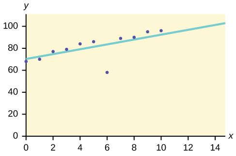
Figure 3.56: Scatterplot that shows a positive, very linear pattern of dots except for one (6, 60). A line of best fit is overlayed on the graph that closely follows the linear dots.
References
Figures
Figure 3.33: Figure 3.10 from OpenStax Statistics (2020) (CC BY 4.0). Retrieved from https://openstax.org/books/statistics/pages/3-5-tree-and-venn-diagrams
Figure 3.34: Figure 3.13 from OpenStax Statistics (2020) (CC BY 4.0). Retrieved from https://openstax.org/books/statistics/pages/3-5-tree-and-venn-diagrams
Figure 3.35: Figure 3.12 from OpenStax Statistics (2020) (CC BY 4.0). Retrieved from https://openstax.org/books/statistics/pages/3-5-tree-and-venn-diagrams
Figure 3.36: Figure 3.14 from OpenStax Statistics (2020) (CC BY 4.0). Retrieved from https://openstax.org/books/statistics/pages/3-5-tree-and-venn-diagrams
Figure 3.37: Figure from OpenStax Statistics (2020) (CC BY 4.0). Retrieved from https://openstax.org/books/statistics/pages/3-5-tree-and-venn-diagrams
Figure 3.38: Figure 3.18 from OpenStax Statistics (2020) (CC BY 4.0). Retrieved from https://openstax.org/books/statistics/pages/3-5-tree-and-venn-diagrams
Figure 3.39: Figure 3.15 from OpenStax Introductory Statistics (2013) (CC BY 4.0). Retrieved from https://openstax.org/books/introductory-statistics/pages/3-solutions#element-750-solution
Figure 3.40: Figure 3.22 from OpenStax Statistics (2020) (CC BY 4.0). Retrieved from https://openstax.org/books/statistics/pages/3-homework
Figure 3.56: Figure 12.24 from OpenStax Introductory Statistics (2013) (CC BY 4.0). Retrieved from https://openstax.org/books/statistics/pages/12-practice
Text
Data from the House Ways and Means Committee, the Health and Human Services Department.
Data from Microsoft Bookshelf.
Data from the United States Department of Labor, the Bureau of Labor Statistics.
Data from the Physician’s Handbook, 1990.
- Haiman, Christopher A., Daniel O. Stram, Lynn R. Wilkens, Malcom C. Pike, Laurence N. Kolonel, Brien E. Henderson, and Loīc Le Marchand. “Ethnic and Racial Differences in the Smoking-Related Risk of Lung Cancer.” The New England Journal of Medicine, 2013. Available online at http://www.nejm.org/doi/full/10.1056/NEJMoa033250 (accessed May 2, 2013). ↵
- "United States: Uniform Crime Report – State Statistics from 1960–2011.” The Disaster Center. Available online at http://www.disastercenter.com/crime (accessed May 2, 2013). ↵
- “Blood Types.” American Red Cross, 2013. Available online at http://www.redcrossblood.org/learn-about-blood/bloodtypes (accessed May 3, 2013). ↵
- Samuel, T. M. “Strange Facts about RH Negative Blood.” Healthfully, 2017. Available online at https://healthfully.com/strange-rh-negative-blood-5552003.html (accessed January 26, 2021). ↵
- Data from the American Cancer Society. ↵
- Data from the Federal Highway Administration, part of the United States Department of Transportation. ↵
- Data from the Federal Highway Administration, part of the United States Department of Transportation. ↵
- Data from Santa Clara County Public Health Department ↵
- Data from United States Senate. Available online at www.senate.gov (accessed May 2, 2013). ↵
- Data from the Baseball-Almanac, 2013. Available online at www.baseball-almanac.com (accessed May 2, 2013). ↵
- Data from the San Jose Mercury News. ↵
