What Is Economics?

To appreciate how a business functions, we need to know something about the economic environment in which it operates. We begin with a definition of economics and a discussion of the resources used to produce goods and services.

Resources: Inputs and Outputs

Economics is the study of the production, distribution, and consumption of goods and services. Resources are the inputs used to produce outputs. Resources may include any or all of the following:

• Land and other natural resources
• Labor (physical and mental)
• Capital, including buildings and equipment
• Entrepreneurship
• Knowledge

Resources are combined to produce goods and services. Land and natural resources provide the needed raw materials. Labor transforms raw materials into goods and services. Capital (equipment, buildings, vehicles, cash, and so forth) are needed for the production process. Entrepreneurship provides the skill, drive and creativity needed to bring the other resources together to produce a good or service to be sold to the marketplace.

Because a business uses resources to produce things, we also call these resources factors of production. The factors of production used to produce a shirt would include the following:

• The land that the shirt factory sits on, the electricity used to run the plant, and the raw cotton from which the shirts are made
• The laborers who make the shirts
• The factory and equipment used in the manufacturing process, as well as the money needed to operate the factory
• The entrepreneurship skills and production knowledge used to coordinate the other resources to make the shirts and distribute them to the marketplace

Input and Output Markets

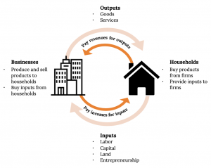
Many of the factors of production are provided to businesses by households. For example, households provide businesses with labor (as workers), land and buildings (as landlords), and capital (as investors). In turn, businesses pay households for these resources by providing them with income, such as wages, rent, and interest. The resources obtained from households are then used by businesses to produce goods and services, which are sold to provide businesses with revenue. The revenue obtained by businesses is then used to buy additional resources, and the cycle continues. This is described in Figure 3.1 “Circular Flow of Inputs and Outputs,” which illustrates the dual roles of households and businesses:

• Households not only provide factors of production (or resources) but also consume goods and services.
• Businesses not only buy resources but also produce and sell both goods and services.

 

Economic Systems

Economists study the interactions between households and businesses and look at the ways in which the factors of production are combined to produce the goods and services that people need. Basically, economists try to answer three sets of questions:

• What goods and services should be produced to meet consumers’ needs? In what quantity? When?
• How should goods and services be produced? Who should produce them, and what resources, including technology, should be combined to produce them?
• Who should receive the goods and services produced? How should they be allocated among consumers?

The answers to these questions depend on a country’s economic system—the means by which a society (households, businesses, and government) makes decisions about allocating resources to produce products and about distributing those products. The degree to which individuals and business owners, as opposed to the government, enjoy freedom in making these decisions varies according to the type of economic system.

Generally speaking, economic systems can be divided into two systems: planned systems and free market systems.

Planned Systems

In a planned system, the government exerts control over the allocation and distribution of all or some goods and services. The system with the highest level of government control is communism. In theory, a communist economy is one in which the government owns all or most enterprises. Central planning by the government dictates which goods or services are produced, how they are produced, and who will receive them. In practice, pure communism is practically nonexistent today, and only a few countries (notably North Korea and Cuba) operate under rigid, centrally planned economic systems.

Under socialism, industries that provide essential services, such as utilities, banking, and health care, may be government owned. Some businesses may also be owned privately. Central planning allocates the goods and services produced by government-run industries and tries to ensure that the resulting wealth is distributed equally. In contrast, privately owned companies are operated for the purpose of making a profit for their owners. In general, workers in socialist economies work fewer hours, have longer vacations, and receive more health care, education, and child-care benefits than do workers in capitalist economies. To offset the high cost of public services, taxes are generally steep. Examples of countries that lean towards a socialistic approach include Venezuela, Sweden, and France.

Free Market System

The economic system in which most businesses are owned and operated by individuals is the free market system, also known as capitalism. In a free market economy, competition dictates how goods and services will be allocated. Business is conducted with more limited government involvement concentrated on regulations that dictate how businesses are permitted to operate. A key aspect of a free market system is the concept of private property rights, which means that business owners can expect to own their land, buildings, machines, etc., and keep the majority of their profits, except for taxes. The profit incentive is a key driver of any free market system. The economies of the United States and other countries, such as Japan, are based on capitalism. However, a purely capitalistic economy is as rare as one that is purely communist. Imagine if a service such as police protection, one provided by government in the United States, were instead allocated based on market forces. The ability to pay would then become a key determinant in who received these services, an outcome that few in American society would consider to be acceptable.

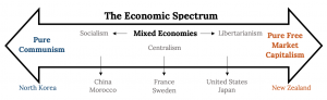
How Economic Systems Compare

In comparing economic systems, it can be helpful to think of a continuum with communism at one end and pure capitalism at the other, as in Figure 3.2 “Economic Spectrum” on the next page. As you move from left to right, the amount of government control over business diminishes. So, too, does the level of social services, such as health care, child-care services, social security, and unemployment benefits. Moving from left to right, taxes are correspondingly lower as well.

 

Mixed Market Economies

Though it’s possible to have a pure communist system, or a pure capitalist (free market) system, in reality many economic systems are mixed. A mixed market economy relies on both markets and the government to allocate resources. In practice, most economies are mixed, with a leaning towards either free market or socialistic principles, rather than being purely one or the other. Some previously communist economies, such as those of Eastern Europe and China, are becoming more mixed as they adopt more capitalistic characteristics and convert businesses previously owned by the government to private ownership through a process called privatization. By contrast, Venezuela is a country that has moved increasingly towards socialism, taking control of industries such as oil and media through a process called nationalization.

The US Economic System

Like most countries, the United States features a mixed market system: though the US economic system is primarily a free market system, the federal government controls some basic services, such as the postal service and air traffic control. The US economy also has some characteristics of a socialist system, such as providing social security retirement benefits to retired workers.

The free market system was espoused by Adam Smith in his book The Wealth of Nations, published in 1776. According to Smith, competition alone would ensure that consumers received the best products at the best prices. In the kind of competition he assumed, a seller who tries to charge more for his product than other sellers would not be able to find any buyers. A job-seeker who asks more than the going wage won’t be hired. Because the “invisible hand” of competition will make the market work effectively, there won’t be a need to regulate prices or wages. Almost immediately, however, a tension developed among free market theorists between the principle of laissez-faire—leaving things alone—and government intervention. Today, it’s common for the US government to intervene in the operation of the economic system. For example, government exerts influence on the food and pharmaceutical industries through the Food and Drug Administration, which protects consumers by preventing unsafe or mislabeled products from reaching the market.

To appreciate how businesses operate, we must first get an idea of how prices are set in competitive markets. The next section, “Perfect Competition and Supply and Demand,” begins by describing how markets establish prices in an environment of perfect competition.

 

Perfect Competition and Supply and Demand

Under a mixed economy, such as we have in the United States, businesses make decisions about which goods to produce or services to offer and how they are priced. Because there are many businesses making goods or providing services, customers can choose among a wide array of products. The competition for sales among businesses is a vital part of our economic system. Economists have identified four types of competition—perfect competition, monopolistic competition, oligopoly, and monopoly. We’ll introduce the first of these—perfect competition—in this section and cover the remaining three in the following section.

Perfect Competition

Perfect competition exists when there are many consumers buying a standardized product from numerous small businesses. Because no seller is big enough or influential enough to affect price, sellers and buyers accept the going price. For example, when a commercial fisher brings his fish to the local market, he has little control over the price he gets and must accept the going market price.

The Basics of Supply and Demand

To appreciate how perfect competition works, we need to understand how buyers and sellers interact in a market to set prices. In a market characterized by perfect competition, price is determined through the mechanisms of supply and demand. Prices are influenced both by the supply of products from sellers and by the demand for products by buyers.

To illustrate this concept, let’s create a supply and demand schedule for one particular good sold at one point in time. Then we’ll define demand and create a demand curve and define supply and create a supply curve. Finally, we’ll see how supply and demand interact to create an equilibrium price—the price at which buyers are willing to purchase the amount that sellers are willing to sell.

Demand and the Demand Curve

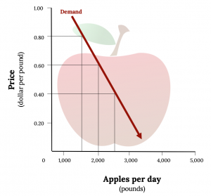
Demand is the quantity of a product that buyers are willing to purchase at various prices. The quantity of a product that people are willing to buy depends on its price. You’re typically willing to buy less of a product when prices rise and more of a product when prices fall. Generally speaking, we find products more attractive at lower prices, and we buy more at lower prices because our income goes further.

Using this logic, we can construct a demand curve that shows the quantity of a product that will be demanded at different prices. Let’s assume that the diagram in Figure 3.3 “Demand Curve” represents the daily price and quantity of apples sold by farmers at a local market. Note that as the price of apples goes down, buyers’ demand goes up. Thus, if a pound of apples sells for $0.80, buyers will be willing to purchase only 1,500 pounds per day. But if apples cost only $0.60 a pound, buyers will be willing to purchase two thousand pounds. At $0.40 a pound, buyers will be willing to purchase 2,500 pounds.

 

Supply and the Supply Curve

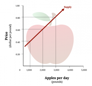
Supply is the quantity of a product that sellers are willing to sell at various prices. The quantity of a product that a business is willing to sell depends on its price. Businesses are more willing to sell a product when the price rises and less willing to sell it when prices fall. Again, this fact makes sense: businesses are set up to make profits, and there are larger profits to be made when prices are high.

Now we can construct a supply curve that shows the quantity of apples that farmers would be willing to sell at different prices, regardless of demand. As you can see in Figure 3.4 “Supply Curve”, the supply curve goes in the opposite direction from the demand curve: as prices rise, the quantity of apples that farmers are willing to sell also goes up. The supply curve shows that farmers are willing to sell only a thousand pounds of apples when the price is $0.40 a pound, two thousand pounds when the price is $0.60, and three thousand pounds when the price is $0.80.

 

Equilibrium Price

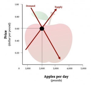
We can now see how the market mechanism works under perfect competition. We do this by plotting both the supply curve and the demand curve on one graph, as we’ve done in Figure 3.5 “Equilibrium Price”. The point at which the two curves intersect is the equilibrium price.

You can see in Figure 3.5 “Equilibrium Price” that the supply and demand curves intersect at the price of $0.60 and quantity of two thousand pounds. Thus, $0.60 is the equilibrium price: at this price, the quantity of apples demanded by buyers equals the quantity of apples that farmers are willing to supply. If a single farmer tries to charge more than $0.60 for a pound of apples, he won’t sell very many because other suppliers are making them available for less. As a result, his profits will go down. If, on the other hand, a farmer tries to charge less than the equilibrium price of $0.60 a pound, he will sell more apples but his profit per pound will be less than at the equilibrium price. With profit being the motive, there is no incentive to drop the price.

 

 

What have we learned in this discussion? Without outside influences, markets in an environment of perfect competition will arrive at an equilibrium point at which both buyers and sellers are satisfied. But we must be aware that this is a very simplistic example. Things are more complex in the real world. For one thing, markets don’t always operate without outside influences. For example, if a government set an artificially low price ceiling on a product to keep consumers happy, we would not expect producers to produce enough to satisfy demand, resulting in a shortage. If government set prices high to assist an industry, sellers would likely supply more of a product than buyers need; in that case, there would be a surplus.

Circumstances also have a habit of changing. What would happen, for example, if incomes rose and buyers were willing to pay more for apples? The demand curve would change, resulting in an increase in equilibrium price. This outcome makes intuitive sense: as demand increases, prices will go up. What would happen if apple crops were larger than expected because of favorable weather conditions? Farmers might be willing to sell apples at lower prices rather than letting part of the crop spoil. If so, the supply curve would shift, resulting in another change in equilibrium price: the increase in supply would bring down prices.

Monopolistic Competition, Oligopoly, and Monopoly

As mentioned previously, economists have identified four types of competition—perfect competition, monopolistic competition, oligopoly, and monopoly. Perfect competition was discussed in the last section; we’ll cover the remaining three types of competition here.

Monopolistic Competition

In monopolistic competition, we still have many sellers, but not nearly as many as we had under perfect competition. And in addition to having fewer sellers, they don’t sell identical products. Instead, they sell differentiated products—products that differ somewhat, or are perceived to differ, even though they serve a similar purpose. Products can be differentiated in a number of ways, including quality, style, convenience, location, and brand name. An example in this case might be toothpaste. Although many people are fiercely loyal to their favorites, most products in this category are quite similar and address the same consumer need. But what if there was a substantial price difference among products? In that case, many buyers would likely be persuaded to switch brands, at least on a trial basis.

How is product differentiation accomplished? Sometimes, it’s simply geographical; you probably buy gasoline at the station closest to your home regardless of the brand. At other times, perceived differences between products are promoted by advertising designed to convince consumers that one product is different from the other—and better than it. Regardless of customer loyalty to a product, if its price goes too high the seller will lose business to a competitor. Therefore, under monopolistic competition, companies have only limited control over price.

Oligopoly

Oligopoly means few sellers. In an oligopolistic market, each seller supplies a large portion of all the products sold in the marketplace. In addition, because the cost of starting a business in an oligopolistic industry is usually high, the number of firms entering it is low. Companies in oligopolistic industries include such large-scale enterprises as automobile companies and airlines. As large firms supplying a sizable portion of a market, these companies have some control over the prices they charge. But there’s a catch: because products are fairly similar, when one company lowers prices, others are often forced to follow suit to remain competitive. You see this practice all the time in the airline industry: When American Airlines announces a fare decrease, Delta, United Airlines, and others do likewise. When one automaker offers a special deal, its competitors usually come up with similar promotions.

Monopoly

In terms of the number of sellers and degree of competition, a monopoly lies at the opposite end of the spectrum from perfect competition. In perfect competition, there are many small companies, none of which can control prices; they simply accept the market price determined by supply and demand. In a monopoly, however, there’s only one seller in the market. The market could be a geographical area, such as a city or a regional area, and doesn’t necessarily have to be an entire country.

There are few monopolies in the United States because the government limits them. Most fall into one of two categories: natural and legal. Natural monopolies include public utilities, such as electricity and gas suppliers. Such enterprises require huge investments, and it would be inefficient to duplicate the products that they provide. They inhibit competition, but they’re legal because they’re important to society. In exchange for the right to conduct business without competition, they’re regulated. For instance, they can’t charge whatever prices they want, but they must adhere to government-controlled prices. As a rule, they’re required to serve all customers, even if doing so isn’t cost efficient.

A legal monopoly arises when a company receives a patent giving it exclusive use of an invented product or process. Patents are issued for a limited time, generally 20 years.^[1] During this period, other companies can’t use the invented product or process without permission from the patent holder. Patents allow companies a certain period to recover the heavy costs of researching and developing products and technologies. A classic example of a company that enjoyed a patent-based legal monopoly is Polaroid, which for years held exclusive ownership of instant-film technology.^[2] Polaroid priced the product high enough to recoup, over time, the high cost of bringing it to market. Without competition, in other words, it enjoyed a monopolistic position in regard to pricing.

 

Measuring the Health of the Economy

Every day, we are bombarded with economic news (at least if you watch the business news stations). We’re told about things like unemployment, home prices, and consumer confidence trends. As a student learning about business, and later as a business manager, you need to understand the nature of the US economy and the terminology that we use to describe it. You need to have some idea of where the economy is heading, and you need to know something about the government’s role in influencing its direction.

Economic Goals

The world’s economies share three main goals:

• Growth
• High employment
• Price stability

Let’s take a closer look at each of these goals, both to find out what they mean and to show how we determine whether they’re being met.

Economic Growth

One purpose of an economy is to provide people with goods and services—cars, computers, video games, houses, rock concerts, fast food, amusement parks. One way in which economists measure the performance of an economy is by looking at a widely used measure of total output called the gross domestic product (GDP). The GDP is defined as the market value of all goods and services produced by the economy in a given year. The GDP includes only those goods and services produced domestically; goods produced outside the country are excluded. The GDP also includes only those goods and services that are produced for the final user; intermediate products are excluded. For example, the silicon chip that goes into a computer (an intermediate product) would not count directly because it is included when the finished computer is counted. By itself, the GDP doesn’t necessarily tell us much about the direction of the economy. But change in the GDP does. If the GDP (after adjusting for inflation, which will be discussed later) goes up, the economy is growing. If it goes down, the economy is contracting.

The Business Cycle

The economic ups and downs resulting from expansion and contraction constitute the business cycle. A typical cycle runs from three to five years but could last much longer. Though typically irregular, a cycle can be divided into four general phases of prosperity, recession, depression (which the cycle generally skips), and recovery:

• During prosperity, the economy expands, unemployment is low, incomes rise, and consumers buy more products. Businesses respond by increasing production and offering new and better products.
• Eventually, however, things slow down. GDP decreases, unemployment rises, and because people have less money to spend, business revenues decline. This slowdown in economic activity is called a recession.
• Economists often say that we’re entering a recession when GDP goes down for two consecutive quarters.
• Generally, a recession is followed by a recovery in which the economy starts growing again.
• If, however, a recession lasts a long time (perhaps a decade or so), while unemployment remains very high and production is severely curtailed, the economy could sink into a depression. Unlike for the term recession, economists have not agreed on a uniform standard for what constitutes a depression, though they are generally characterized by their duration. Though not impossible, it’s unlikely that the United States will experience another severe depression like that of the 1930s. The federal government has a number of economic tools (some of which we’ll discuss shortly) with which to fight any threat of a depression.

Full Employment

To keep the economy going strong, people must spend money on goods and services. A reduction in personal expenditures for things like food, clothing, appliances, automobiles, housing, and medical care could severely reduce GDP and weaken the economy. Because most people earn their spending money by working, an important goal of all economies is making jobs available to everyone who wants one. In principle, full employment occurs when everyone who wants to work has a job. In practice, we say that we have full employment when about 95 percent of those wanting to work are employed.

The Unemployment Rate

The US Department of Labor tracks unemployment and reports the unemployment rate: the percentage of the labor force that’s unemployed and actively seeking work. The unemployment rate is an important measure of economic health. It goes up during recessionary periods because companies are reluctant to hire workers when demand for goods and services is low. Conversely, it goes down when the economy is expanding and there is high demand for products and workers to supply them.

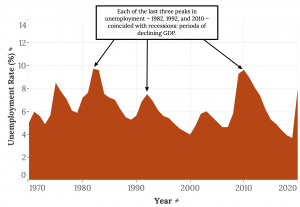
Figure 3.6 “US Unemployment Rate, 1970-2020” traces the US unemployment rate between 1970 and 2020. Please be aware that there are multiple measures of unemployment and that this graph is based on what is known as U3, the most commonly used measurement. Another measurement, U6, is considered to provide a broader picture of unemployment in the United States. It includes two groups of people that U3 doesn’t: those who are not actively looking for work but would like a job and have looked for one in the last 12 months; and those who would like to work full-time jobs but have settled for part-time positions because full-time work was not available to them. Since by definition, U6 is always higher than U3, it is likely that U3 is discussed more often because it paints a more favorable, if not completely accurate, picture.

 

Price Stability

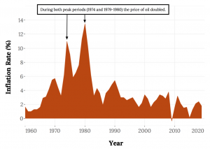
A third major goal of all economies is maintaining price stability. Price stability occurs when the average of the prices for goods and services either doesn’t change or changes very little. Rapidly rising prices are troublesome for both individuals and businesses. For individuals, rising prices mean people have to pay more for the things they need. For businesses, rising prices mean higher costs, and, at least in the short run, businesses might have trouble passing on higher costs to consumers. When the overall price level goes up, we have inflation. Figure 3.7 “US Inflation Rate, 1960-2020” shows inflationary trends in the US economy since 1960. When the price level goes down (which rarely happens), we have deflation. A deflationary situation can also be damaging to an economy. When purchasers believe they can expect lower prices in the future, they may defer making purchases, which has the effect of slowing economic growth (GDP) accompanied by a rise in unemployment. Japan experienced a long period of deflation which contributed to economic stagnation in that country from which it is only now beginning to recover.

 

The Consumer Price Index

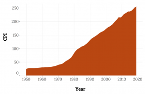
The most widely publicized measure of inflation is the consumer price index (CPI), which is reported monthly by the Bureau of Labor Statistics. The CPI measures the rate of inflation by determining price changes of a hypothetical basket of goods, such as food, housing, clothing, medical care, appliances, automobiles, and so forth, bought by a typical household.

The CPI base period is 1982 to 1984, which has been given an average value of 100. Figure 3.8 “Selected CPI Values, 1950-2019” gives CPI values computed for selected years. The CPI value for 1950, for instance, is 24. This means that $1 of typical purchases in 1982 through 1984 would have cost $0.24 in 1950. Conversely, you would have needed $2.18 to purchase the same $1 worth of typical goods in 2010. The difference registers the effect of inflation. In fact, that’s what an inflation rate is—the percentage change in a price index.

 

Economic Forecasting

In the previous section, we introduced several measures that economists use to assess the performance of the economy at a given time. By looking at changes in the GDP, for instance, we can see whether the economy is growing. The CPI allows us to gauge inflation. These measures help us understand where the economy stands today. But what if we want to get a sense of where it’s headed in the future? To a certain extent, we can forecast future economic trends by analyzing several leading economic indicators.

Economic Indicators

An economic indicator is a statistic that provides valuable information about the economy. There’s no shortage of economic indicators, and trying to follow them all would be an overwhelming task. So in this chapter, we’ll only discuss the general concept and a few of the key indicators.

Lagging and Leading Indicators

Economists use a variety of statistics to discuss the health of an economy. Statistics that report the status of the economy looking at past data are called lagging economic indicators. This type of indicator looks at trends to determine how strong an economy is and its direction. One such indicator is average length of unemployment. If unemployed workers have remained out of work for a long time, we may infer that the economy has been slow. Another lagging indicator is GDP growth. Even if the last several quarters have followed the same trend, though, there is no way to say with confidence that such a trend will necessarily continue.

Indicators that predict the status of the economy three to twelve months into the future are called leading economic indicators. If such an indicator rises, the economy is more likely to expand in the coming year. If it falls, the economy is more likely to contract. An example of a leading indicator is the number of permits obtained to build homes in a particular time period. If people intend to build more homes, they will be buying materials like lumber and appliances, and also employ construction workers. This type of indicator has a direct predictive value since it tells us something about what level of activity is likely in a future period.

In addition to housing, it is also helpful to look at indicators from sectors like labor and manufacturing. One useful indicator of the outlook for future jobs is the number of new claims for unemployment insurance. This measure tells us how many people recently lost their jobs. If it’s rising, it signals trouble ahead because unemployed consumers can’t buy as many goods and services as they could if they had paychecks. To gauge the level of goods to be produced in the future (which will translate into future sales), economists look at a statistic called average weekly manufacturing hours. This measure tells us the average number of hours worked per week by production workers in manufacturing industries. If it’s on the rise, the economy will probably improve.

Since employment is such a key goal in any economy, the Bureau of Labor Statistics tracks total non-farm payroll employment from which the number of net new jobs created can be determined.

The Conference Board also publishes a consumer confidence index based on results of a monthly survey of five thousand US households. The survey gathers consumers’ opinions on the health of the economy and their plans for future purchases. It’s often a good indicator of consumers’ future buying intent.

 

Government’s Role in Managing the Economy

Monetary Policy

Monetary policy is exercised by the Federal Reserve System (“the Fed”), which is empowered to take various actions that decrease or increase the money supply and raise or lower short-term interest rates, making it harder or easier to borrow money. When the Fed believes that inflation is a problem, it will use contractionary policy to decrease the money supply and raise interest rates. When rates are higher, borrowers have to pay more for the money they borrow, and banks are more selective in making loans. Because money is “tighter”—more expensive to borrow—demand for goods and services will go down, and so will prices. In any case, that’s the theory.

The Fed will typically tighten or decrease the money supply during inflationary periods, making it harder to borrow money.

To counter a recession, the Fed uses expansionary policy to increase the money supply and reduce interest rates. With lower interest rates, it’s cheaper to borrow money, and banks are more willing to lend it. We then say that money is “easy.” Attractive interest rates encourage businesses to borrow money to expand production and encourage consumers to buy more goods and services. In theory, both sets of actions will help the economy escape or come out of a recession.

Fiscal Policy

Fiscal policy relies on the government’s powers of spending and taxation. Both taxation and government spending can be used to reduce or increase the total supply of money in the economy—the total amount, in other words, that businesses and consumers have to spend. When the country is in a recession, government policy is typically to increase spending, reduce taxes, or both. Such expansionary actions will put more money in the hands of businesses and consumers, encouraging businesses to expand and consumers to buy more goods and services. When the economy is experiencing inflation, the opposite policy is adopted: the government will decrease spending or increase taxes, or both. Because such contractionary measures reduce spending by businesses and consumers, prices come down and inflation eases.

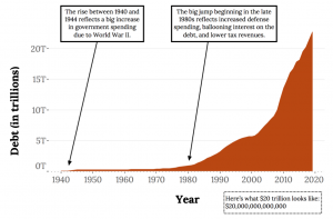
The National Debt

If, in any given year, the government takes in more money (through taxes) than it spends on goods and services (for things such as defense, transportation, and social services), the result is a budget surplus. If, on the other hand, the government spends more than it takes in, we have a budget deficit (which the government pays off by borrowing through the issuance of Treasury bonds). Historically, deficits have occurred much more often than surpluses; typically, the government spends more than it takes in. Consequently, the US government now has a total national debt of more than $19 trillion (Note: This number is moving too quickly for the authors to keep the graph current—you can see the current debt at http://www.usdebtclock.org/).

 

 

 

Chapter Video 

This video presents a balanced view of capitalism and socialism and reinforces key points within the chapter. Since it is rather dry, it would be fine to watch only the first seven minutes or so.

(Copyrighted material)

Image Credits: Chapter 3

Figure 3.1: Alex Muravev. “House.” Noun Project Inc. Retrieved from: https://thenounproject.com/search/?q=house&i=983462; Graphiqu. “City Building.” Noun Project Inc. Retrieved from: https://thenounproject.com/search/?q=city building&i=2579723

Figure 3.3: Sanja (2013). “Simple Red Apple.” OpenClipArt. Public Domain. Retrieved from: https://openclipart.org/detail/183893/simple-red-apple

Figure 3.4: Sanja (2013). “Simple Red Apple.” OpenClipArt. Public Domain. Retrieved from: https://openclipart.org/detail/183893/simple-red-apple

Figure 3.5: Sanja (2013). “Simple Red Apple.” OpenClipArt. Public Domain. Retrieved from: https://openclipart.org/detail/183893/simple-red-apple

Figure 3.6: U.S. Bureau of Labor Statistics. “The U.S. Unemployment Rate, 1970-2020.” Data Retrieved from: https://data.bls.gov/timeseries/LNS14000000

Figure 3.7: US Inflation Calculator. “The US inflation rate, 1960-2020.” Data Retrieved from: https://www.usinflationcalculator.com/inflation/historical-inflation-rates/

Figure 3.8: US Inflation Calculator. “Selected CPI Values, 1950-2019.” Data Retrieved from: https://www.usinflationcalculator.com/inflation/consumer-price-index-and-annual-percent-changes-from-1913-to-2008/

Figure 3.9: Treasury Direct. “The National Debt, 1940-2019.” Data Retrieved from: https://www.treasurydirect.gov/govt/reports/pd/histdebt/histdebt_histo3.htm

Video Credits: Chapter 3

Guyus Seralius (2013, February 20). “Capitalism vs Socialism-A Balanced Approach.” YouTube. Retrieved from: https://www.youtube.com/watch?v=PBIXmXJwIuk