Chapter 9. The Role of Performance in Aircraft Design: Constraint Analysis
Introduction
In the proceeding chapters we have looked at many aspects of basic aircraft performance. These included takeoff and landing, turns, straight and level flight in cruise, and climb. If we were to look at the relationships we found for any of these we could see how we might design an airplane to best accomplish the task at hand. In other words, if we wanted to design an aircraft that could takeoff and land in a very short distance we can look at the takeoff and landing distance equations and identify the factors that would minimize these distances. To takeoff in a short distance we might want a high maximum lift coefficient to get a low takeoff speed, a large wing area to give a lot of lift at low speed, and a lot of thrust to accelerate to takeoff distance in as short a ground run as possible. To land in a short distance we might want to also design a plane with a large wing and high maximum lift coefficient but now the thrust isn’t as important as the amount of braking friction available unless it is reverse thrust that we are talking about.
Of course there are limits to be considered. High thrust will minimize the takeoff ground run but once thrust becomes as high as the weight of the plane we might as well take off vertically! And a big wing area gives us high drag along with high lift. Nonetheless, we can see that three parameters; thrust, weight, and wing area, are important factors to consider in takeoff.
We would find, if we looked at the equations we derived for the other types of flight mentioned above that these same three parameters pop up everywhere. The only problem is that we would find that their relationships in cruise aren’t necessarily the same as they are in takeoff and landing. And they may be different still in climb.
If we want an airplane that only does one thing well we need only look at that one thing. If, for example, we went all out to create a plane that could takeoff in a very short distance and then look at its performance in straight and level cruise we would probably find that it isn’t very good. And its climbing performance may be even worse!
This isn’t really much different from designing any other product that is capable of more than one task. A car can be designed to go really fast or to get really good gas mileage, but probably not both. Car tires can be designed to have high traction in mud and snow or to give great mileage at highway speeds but any attempt to design an “all weather touring” tire will result in a compromise with less traction than a mud and snow tire and poorer performance at high speeds than the high speed highway tire design.
The question with the design of an airplane as with a car or a tire, is how do we arrive at the best compromise that will result in a good all around design while still being better than average in one or two desired areas?
One way to approach this would be to go back to the equations in earlier chapters and iterate among them, trying to find wing areas, weights, and engine sizes that would accomplish our design objectives. We might start with cruise since a certain minimum range is often a design objective. We know that in cruise since lift must equal weight, we can select a design value of cruise lift coefficient (commonly around 0.2 to 0.3) and a desired cruise speed and altitude and solve for the needed wing area.
S = 2W/(ρV2CL)
If our desire is to look at an optimum range we might want to find the ratio of lift to drag that will maximize range (for example, for a propeller driven plane Rmax occurs with flight at [L/D]max or at minimum drag conditions). Finding this value of drag would set the thrust we need for cruise. Within all this we could look at the effects of aspect ratio and Oswald’s efficiency factor to find how wing planform shape will affect our results.
In this manner, we can find values of weight, wing area, and thrust that match our desired cruise capability. However, these may not represent the best combination of these parameters if another of our goals is to achieve a certain climb rate.
Another factor to consider would be the desired maximum speed at the cruise altitude. This can be put into the drag equation with the numbers found above to get the thrust or power needed to reach that maximum speed.
The cruise based calculations mentioned above would give us valuable design information for our airplane based on a desired cruise speed and altitude for a design weight and would tell us the wing area and thrust needed for that cruise condition and the thrust needed to cruise at a desired maximum speed. It would not, however tell us if this would result in a good ability to climb or the ability to takeoff and land in a reasonable distance. We would also need to look at these requirements and our design objectives.
To see if we can climb at the desired rate over a reasonable range of altitudes we would need to look at the climb relationship:
dh/dt = [Pavail – Preq] / W
This would give us another value of thrust needed to reach the target rate of climb for a given weight and, since the equation contains power required, which is drag times speed, the wing area would also be a factor.
Finally, we would need to look at the takeoff and landing relationships and at our target values for ground run or for the total takeoff or landing distance. These relationships also involve thrust, weight, and wing area.
The essence of all this is that if we even have only three primary design objectives; a cruise specification, a climb requirement, and a takeoff or landing constraint, we can end up with three different values for wing area and thrust required for a given aircraft weight. We would then have to decide which of these three requirements was most important and which was least important and then start varying design parameters in an iterative manner until we got all three objectives to result in the same weight, wing area, and engine thrust.
This process would become even more cumbersome as we added other design objectives such as a minimum turning radius or a minimum stall speed.
The question is; is there some way to analyze all of these at the same time and come to a decision about optimum or reasonable compromise values of weight, wing area, and engine thrust without having to go through iteration after iteration? Fortunately, the answer is yes. The method normally used is called “constraint analysis”.
9.1 Constraint Analysis
Constraint analysis is essentially a way to look at aircraft weight, wing area, and engine thrust for various phases of flight and come to a decision about meaningful starting values of all three parameters for a given set of design objectives. It does this by looking at two important ratios, the thrust-to-weight ratio (T/W), the wing loading or ratio of weight-to-planform area (W/S). Or in some cases the power-to-weight ratio (P/W) is used instead of T/W. These two ratios are both very reflective of the design philosophy and objectives of any particular airplane.
As one of my students once put it, the thrust-to-weight ratio (T/W) is a measure of how much of a rocket your plane is. The more efficient a plane is in things like cruise the lower its value of T/W. The limit is a sailplane with T/W = 0 and at the other extreme we have fighter aircraft where T/W approaches unity. If T/W = 1.0 or greater we need no wing. The vehicle can get into the air with no lift at all. The value of T/W will depend on the desired flight speed, the wing area, and the efficiency (L/D) of the wing. In cruise where lift = weight and thrust = drag, T/W = 1 / [L/D], meaning that the high value of L/D that is needed for a large range goes hand in hand with a low thrust-to-weight ratio.
The other parameter, W/S, or wing loading, is also generally low for sailplanes and high for fighters. Wing loading for sailplanes is usually in the range of 5-8 pounds per square foot, around 17 lb/ft2 for general aviation planes, and over 100 lb/ft2 for fighters. This ratio is a measure of aerodynamic efficiency as well as a measure of the way the structure is designed.
These two ratios are tied together in aircraft performance through the same power relationship that we looked at when we first examined climb and glide.
9.2 Specific Excess Power
In an earlier chapter on climb and glide we looked at something called specific excess power and defined it as:
Ps = [Pavail – Preq] / W = [(T – D)V] / W
We may, hopefully, remember using this relationship to find the rate of climb but we may not recall that it was only the correct rate of climb in a special case, where speed (V) was constant; i.e., the static rate of climb:
[dh/dt]static = [(T – D)V] / W
If we go back to that earlier chapter we will find that in a more general relationship we had:
Ps = [Pavail – Preq] / W = [(T – D)V] / W = [dh/dt] + (V/g)(dV/dt).
In other words, only when velocity (V) is constant is this relationship strictly equal to the rate of climb.
In reality, the specific excess power relationship tells us how the excess engine power, Pavail – Preq , can be used to increase the aircraft’s potential energy (climb) or its kinetic energy (speed). In other words this equation is really an energy balance. Power required is the power needed to maintain straight and level flight, i.e., to overcome drag and to go fast enough to give enough lift to equal the weight. If the engine is capable of producing more power than the power required, that excess power can be used to make the plane accelerate to a faster speed (increasing kinetic energy) or to climb to a higher altitude (increasing potential energy), or to give some combination of both. It can tell us how much speed we can gain by descending to a lower altitude, converting potential energy to kinetic energy, or how we can perhaps climb above the static ceiling of the aircraft by converting excess speed (kinetic energy) into extra altitude (potential energy).
In essence this is a pretty powerful relationship and it can be used to analyze many flight situations and to determine an airplane’s performance capabilities. Let’s look at how the equation can be rearranged to help us examine the performance needs in various types of flight.
Rearranging the equation we have:
(T/W)V = (D/W)V +dh/dt + (V/g)(dV/dt)
Now we can expand the first term on the right hand side by realizing that
D = (CD0 + kCL2) ½ ρV2S.
Substituting this for drag in the equation and dividing the entire equation by V we can get:
(T/W) = [(CD0 + kCL2) ½ ρV2S) /W] + (1/V)dh/dt + (1/g)(dV/dt)
Now, to simplify things a little we are going to use a common substitution for the dynamic pressure:
q = ½ ρV2 .
We will also define the lift coefficient in terms of lift and weight using the most general form where in a turn or other maneuver lift may be equal to the load factor n times the weight.
CL = L / qS = nW / qS
Putting all of this together will give:
T/W = (qCD0)/(W/S) + (kn2/q)(W/S) + (1/V)dh/dt + (1/g)dV/dt
In the equation above we have a very general performance equation that can deal with changes in both speed and altitude and we find that these changes are functions of the thrust-to-weight ratio, T/W, and the wing loading W/S. Note that just as the drag equation is a function of both V and 1/V, this is a function of both W/S and 1/(W/S).
9.3 Straight and level flight
We can use the above relationship to make plots of the thrust-to-weight ratio versus the wing loading for various types of flight. If, for example, we want to look at conditions for straight and level flight we can simplify the equation knowing that:
Straight and level flight: n = 1, dh/dt = 0, dV/dt = 0, giving:
T/W = (qCD0)/(W/S) + (k/q)(W/S)
So for a given estimate of our design’s profile drag coefficient, aspect ratio, and Oswald efficiency factor [ k = 1/(πARe)] we can plot T/W versus W/S for any selected altitude (density) and cruise speed.
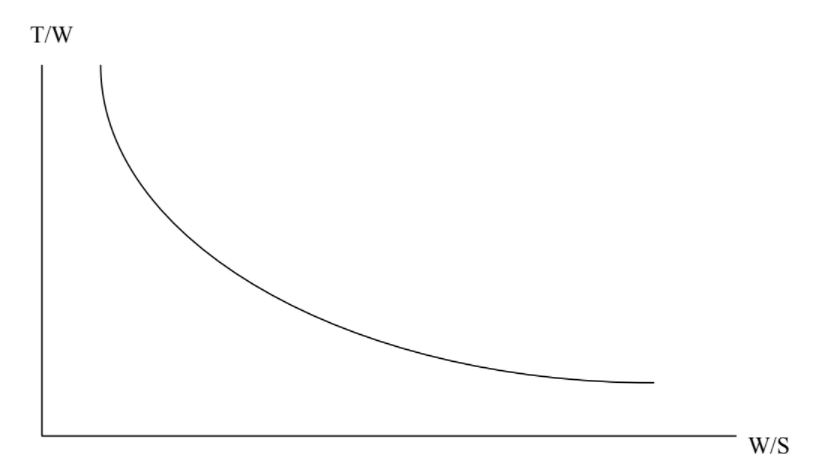
We could get a different curve for different cruise speeds and altitudes but at any given combination of these this will tell us all the combinations of thrust-to-weight values and wing loadings that will allow straight and level flight at that altitude and speed.
In understanding what this really tells us we perhaps need to step back and look at the same situation another way. In straight and level flight we know:
L = W = qSCL
and T = D = qS (CD0 + kCL2)
And if we simply combine these two equations we will get the same relationship we plotted above.
T/W = (qCD0)/(W/S) + (k/q)(W/S)
Hence, what we have done through the specific excess power relationship is nothing but a different way to get a familiar result. We just end up writing that result in a different form, in terms of the thrust-to-weight ratio and the wing loading.
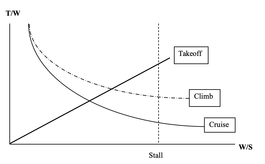
We need to note that to make the plot above we had to choose a cruise speed. We need to keep in mind that there are limits to that cruise speed. We can’t fly straight and level at speeds below the stall speed or above the maximum speed where the drag equals the maximum thrust from the engine. We could put these limits on the same plot if we wish. For example, let’s look at stall.
At stall Vstall = [2W/(ρSCLmax)]1/2
And this can be written [W/S] = ½ ρVstall2CLmax
On the plot above this would be a vertical line, looking something like this
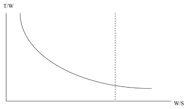
Here we should note that the space to the right of the dashed line for stall is “out of bounds” since to fly here would require a higher maximum lift coefficient.
9.4 Climb
We could return to the reorganized excess power relationship
T/W = (qCD0)/(W/S) + (kn2/q)(W/S) + (1/V)dh/dt + (1/g)dV/dt
and look at steady state climb. For climb at constant speed dV/dt = 0 and our equation becomes
T/W = (qCD0)/(W/S) + (kn2/q)(W/S) + (1/V)dh/dt
and we can plot T/W versus W/S just as we did in the cruise case, this time specifying a desired rate of climb along with the flight speed and other parameters. Doing this will add another curve to our plot and it might look like the figure below.
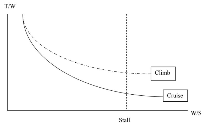
This addition to the plot tells us the obvious in a way. It says that we need a higher thrust-to-weight ratio to climb than to fly straight and level.
Each plot of the specific power equation that we add to this gives us a better definition of our “design space”. It tells us that to make the airplane do what we want it to do we are restricted to certain combinations of T/W and W/S.
9.4.1 Caution
It should be noted that in plotting curves for cruise and climb a flight speed must be selected for each. It is, for example, a common mistake for students to look at the performance goals for an aircraft design and just plug in the numbers given without thinking about them. Design goals might include a maximum speed in cruise of 400 mph and a maximum range goal of 800 miles, however these do not occur at the same flight conditions. Just as a car cannot get its best gas mileage when the car is moving at top speed, an airplane isn’t going to get maximum range at its top cruise speed. In fact, the equations used to find the maximum range for either a jet or a prop aircraft assume flight at very low speeds, speeds that one would never really use in cruise unless desperate to extend range in some emergency situation. When plotting the cruise curve in a constraint analysis plot it should be assumed that the aircraft is cruising at a desired “normal” cruise speed, which will be neither the top speed at that altitude nor the speed for maximum range. As an example, most piston engine aircraft will cruise at an engine power setting somewhere between 55% and 75% of maximum engine power. On the other hand, the climb curve should be plotted for optimum conditions; i.e., maximum rate of climb (minimum power required conditions for a prop aircraft) since that is the design target in climb.
9.5 Altitude effects
Obviously altitude is a factor in plotting these curves. The cruise curve will normally be plotted at the desired design cruise altitude. The climb curve would probably be plotted at sea level conditions since that is where the target maximum rate of climb is normally specified. This presents somewhat of a problem since we are plotting the relationships in terms of thrust and weight and thrust is a function of altitude while weight is undoubtedly less in cruise than at takeoff and initial climb-out. One way to resolve this issue is to write our equations in terms of ratios of thrust at altitude divided by thrust at sea level and weight at altitude divided by weight at takeoff.
Talt / Tsl and Walt / WTO .
Going back to our main equation:
T/W = (qCD0)/(W/S) + (kn2/q)(W/S) + (1/V)dh/dt + (1/g)dV/dt ,
we rewrite this in terms of the ratios above to allow us to make our constraint analysis plots functions of TSL and WTO.
TSL / WTO = [(Walt/WTO) / (Talt/TSL)] {[q/(Walt/WSL)](CD0)/(WTO/S)
+ (kn2/q)(WTO/S)(Walt/WTO) + (1/V)dh/dt + (1/g)dV/dt} .
Some references give these ratios, which have been italicized above, symbols such as α and β to make the equation look simpler.
Note that the thrust ratio above is normally just the ratio of density since it is normally assumed that
Talt / Tsl = ρalt / ρSL .
9.6 Other Design Objectives Including Take-off
What other design objectives can be added to the constraint analysis plot to further define our design space? One that is fairly easy to deal with is turning.
Often a set of design objectives will include a minimum turn radius or minimum turn rate. If we assume a coordinated turn we find that once again the last two terms in the constraint analysis relationship go to zero since a coordinated turn is made at constant altitude and airspeed. All we need to do is go to the turn equations and find the desired airspeed and load factor (n), put these into the equation and plot it. Normally we would look at turns at sea level conditions and at takeoff weight. This would give a curve that looks similar to the plots for cruise and climb.
The plot that will be different from all of these is that for takeoff. The takeoff equation seen in an earlier chapter is somewhat complex because takeoff ground distances depend on many things, from drag coefficients to ground friction.
STO = (1/2B) ln [A /(A – BVTO2)]
where A = g[(T0/W) – μ]
and B = (g/W) [ ½ ρS(CD – μCLg) + a] .
It should be recalled that CLg is the value of lift coefficient during the ground roll, not at takeoff, and its value is μ/2k for the theoretically minimum ground run. The last parameter in the “B” equation above is “a”, a term that appears in the thrust equation:
T = T0 –aV2 ,
a relationship that comes from the momentum equation where T0 is the “static thrust” or the thrust when the airplane is standing still.
It can be noted that in the A and B terms respectively we have the thrust-to-weight ratio and the inverse of the wing loading (W/S); hence, for a given set of takeoff parameters and a desired ground run distance (STO) a plot can be made of T/W versus W/S. This relationship proves to be a little messy with both ratios buried in a natural log term and the wing loading in a separate term. An iterative solution may be necessary.
An alternative approach often proposed in books on aircraft design is based on statistical takeoff data collected on different types of aircraft. The figure below (Raymer, 1992) is based on a method commonly used in industry.
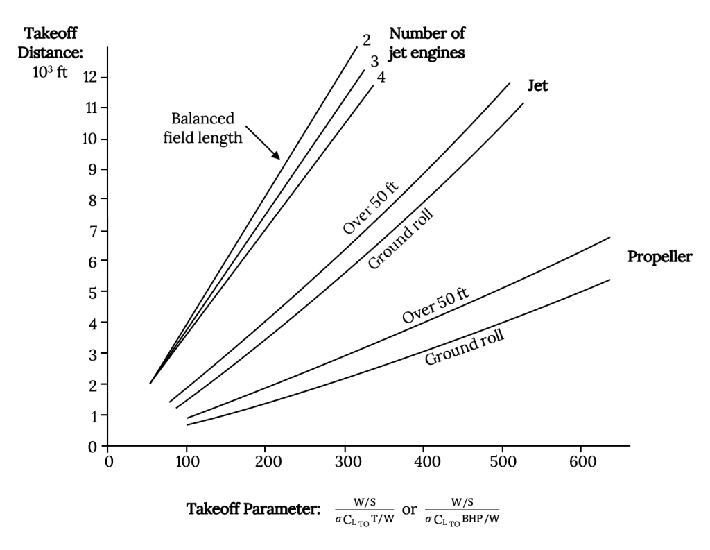
In this approach a “Take-Off-Parameter”, TOP, is proposed to be a function of W/S, T/W, CLTO, and the density ratio sigma (σ) where:
W/S = (TOP)σCLTO(T/W). [σ = ρalt/ρSL]
The value of “TOP” is found from the chart above. One finds the desired takeoff distance in feet on the vertical axis and projects over to the plot for the type of aircraft desired, then drops a vertical line to the TOP axis to find a value for that term. Once the value of TOP has been found the relationship above is plotted to give a straight line from the origin of the constraint analysis graph.
Two things should be noted at this point. First is that the figure from Raymer on the preceding page has two types of plots on it, one for ground run only and the other for ground run plus the distance required to clear a 50 ft obstacle. Either can be used depending on the performance parameter which is most important to meeting the design specifications. The second is that the takeoff parameter (TOP) defined for propeller aircraft is based on power requirements (specifically, horsepower requirements) rather than thrust. For the prop aircraft Raymer defines TOP as follows:
W/S = (TOP)σCLTO(hp/W) .
It should be noted here that it is often common when conducting a constraint analysis for a propeller type aircraft to plot the power-to-weight ratio versus wing loading rather than using the thrust-to-weight ratio. This can be done fairly easily by going back to the constraint analysis equations and substituting P/V everywhere that a thrust term appears.
9.7 Landing
In reality, the landing distance is pretty much determined by the stall speed (the plane must touch down at a speed higher than stall speed, often about 1.2 VStall) and the glide slope (where obstacle clearance is part of the defined target distance). Again it is common for aircraft design texts to propose approximate or semi-empirical relationships to describe this and those relationships show landing distance to depend only on the wing loading. This makes sense when one realizes that, unless reverse thrust is used in the landing ground run, thrust does not play a major role in landing. Raymer proposed the relationship below:
Slanding = 80(W/S)[1/(σCLmax)] + Sa
where
Sa = 1000 for an airliner with a 3 degree glideslope
600 for a general aviation type power off approach
450 for a STOL 7 degree glideslope
Raymer also suggests multiplying the first term on the right in the distance equation above by 0.66 if thrust reversers are to be used and by 1.67 when accounting for the safety margin required for commercial aircraft operating under FAR part 25.
Note here that the weight in the equation is the landing weight but that in calculating this landing distance for design purposes the takeoff weight is usually used for general aviation aircraft and trainers and is assumed to be 0.85 times the takeoff weight for jet transports.
The relationship above, since it does not depend on the thrust, will plot on our constraint analysis chart as a vertical line in much the same way the stall case did, but it will be just to the left of the stall line.
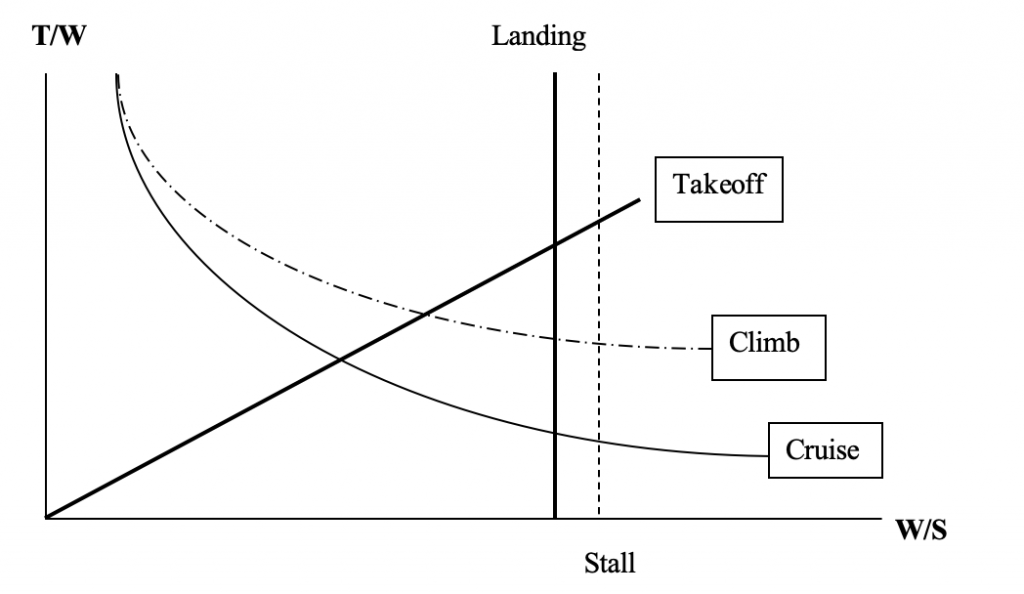
9.8 Optimum design points
In this final plot the space above the climb and takeoff curves and to the left of the landing line is our acceptable design space. Any combination of W/S and T/W within that space will meet our design goals. What we want, however, is the “best” combination of these parameters for our design goals. The optimum will be found at the intersections of these curves. In the figure above this will be either where the takeoff and climb curves intersect or where the takeoff and landing curves intersect.
By “optimum” we mean that we are looking for the minimum thrust-to-weight ratio that will enable the airplane to meet its performance goals and we would like to have the highest possible wing loading. The desire for minimum thrust is obvious, based on the need to minimize fuel consumption and engine cost. The goal of maximum wing loading may not be as obvious to the novice designer but this means the wing area is kept to a minimum which gives lower drag. It also gives a better “ride” to the airplane passengers. As wing loading increases the effects of turbulence and gusts in flight are minimized, smoothing out the “bumps” in flight.
9.9 The design process
Constraint analysis is an important element in a larger process called aircraft design. There are many good textbooks available on aircraft design and the Raymer text referenced earlier is one of the best. Another good text that combines an examination of the design process with a look as several design case studies is Aircraft Design Projects for Engineering Students, by Jenkinson and Marchman, published by the AIAA.
The design process usually begins with a set of design objectives such as these we have examined, a desired range, payload weight, rate of climb, takeoff and landing distances, top speed, ceiling, etc. The first step in the process is usually to look for what are called “comparator” aircraft, existing or past aircraft that can meet most or all of our design objectives. This data can give us a place to start by suggesting starting values of things like takeoff weight, wing area, aspect ratio, etc. that can be used in the constraint analysis equations above. These are then plotted to find “optimum” values of wing loading and thrust-to-weight ratio.
The constraint analysis may be performed several times, looking at the effects of varying things like wing aspect ratio on the outcome. The analysis may suggest that some of the “constraints” (i.e., the performance targets) need to be relaxed. What can be gained by accepting a lower cruise speed or a longer takeoff distance. We might find, for example, that by accepting an additional 500 feet in our takeoff ground run we can get by with a significantly smaller engine.
Design is a process of compromise and no one design is ever best at everything. But through good use of things like constraint analysis methods we can turn those compromises into optimum solutions.
Acknowledgment: Thanks to Dustin Grissom for reviewing the above and developing examples to go with it.
Homework 9
Looking again at the aircraft in Homework 8 with some additional information:
| Cessna 182 | Cessna Citation III |
|---|---|
| b = 35.8 ft | b = 53.3 ft |
| S = 174 ft^2 | S = 318 ft^2 |
| W_max = 2950 lb | W_max = 19,815 lb |
| Fuel = 65 gal (@ 6 lb/gal) | Fuel = 1119 gal (@ 6.67 lb/gal) |
| Single engine 230 hp at SL | 2 engines with 3650 lb thrust each at SL |
| eta_p = 0.8 | |
| gamma_p = 0.45 lb/hp-hr | gamma_T = 0.6 lb/lb_thrust-hr |
| C_D0 = 0.025 | C_Do = 0.02 |
| e = 0.8 | e = 0.81 |
1. Find the maximum range and the maximum endurance for both aircraft.
a. What altitude gives the best range for the C-182? Do you think this is a reasonable speed for flight?
b. What altitude gives the best endurance for the C-182? Is this a reasonable flight speed?
c. Endurance for the C-182 can be found two ways (constant altitude or constant velocity). Which gives the best endurance?
2. Find the range for the C-182 assuming the flight starts at 150 mph and an altitude of 7500 feet and stays at constant angle of attack.
3. How sensitive is the maximum range for the Cessna 182 to aspect ratio and the Oswald efficiency factor, i.e. to the wing planform shape? To answer this, plot range versus aspect ratio using e.= 0.8 and varying AR from 4 through 10, and plot range versus e for an aspect ratio of 7.366 with e varying from 0.6 through 1.0.
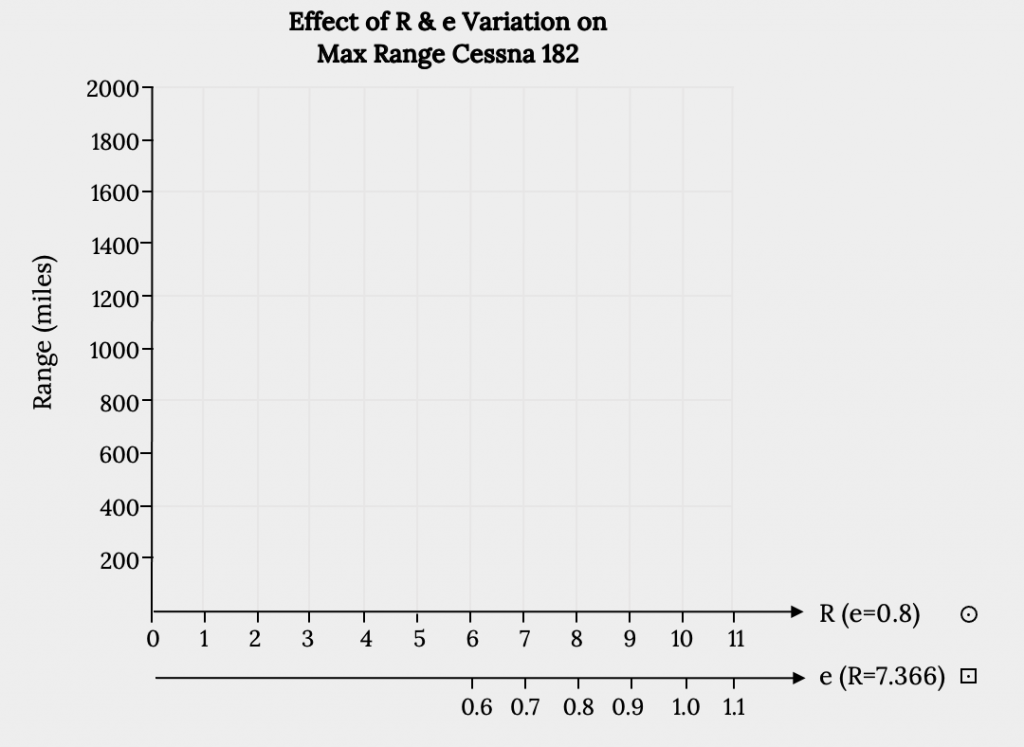
Figure 9.7: Effect of R & e Variation on max Range Cessna 182
References
Raymer, Daniel P. (1992). Aircraft Design: A Conceptual Approach, AIAA, Washington, DC.
Figure 9.1: James F. Marchman (2004). “Inverse Relationship between Thrust to Weight Ratio and Weight to Surface Area Ratio.” CC BY 4.0.
Figure 9.2: James F. Marchman (2004). “Stall Cutoff for cap W over cap S values.” CC BY 4.0.
Figure 9.3: James F. Marchman (2004). “Effects of a Desired Climb Rate on Aircraft Design Space.” CC BY 4.0.
Figure 9.4: Kindred Grey (2021). “Effect of Aircraft Parameters on Takeoff Distance.” CC BY 4.0. Adapted from Raymer, Daniel P. (1992). Aircraft Design: A Conceptual Approach, AIAA, Washington, DC. Available from https://archive.org/details/9.4_20210805
Figure 9.5: James F. Marchman (2004). “Effect of Desired Takeoff Characteristics on Aircraft Design Space.” CC BY 4.0.
Figure 9.6: James F. Marchman (2004). “Effect of Desired Landing Characteristics on Aircraft Design Space.” CC BY 4.0.
Figure 9.7: Kindred Grey (2021). “Effect of R & e Variation on max Range Cessna 182.” CC BY 4.0. Adapted from James F. Marchman (2004). CC BY 4.0. Available from https://archive.org/details/hw-9_20210805
