Chapter 4. Performance in Straight and Level Flight
Introduction
Now that we have examined the origins of the forces which act on an aircraft in the atmosphere, we need to begin to examine the way these forces interact to determine the performance of the vehicle. We know that the forces are dependent on things like atmospheric pressure, density, temperature and viscosity in combinations that become “similarity parameters” such as Reynolds number and Mach number. We also know that these parameters will vary as functions of altitude within the atmosphere and we have a model of a standard atmosphere to describe those variations. It is also obvious that the forces on an aircraft will be functions of speed and that this is part of both Reynolds number and Mach number.
Many of the questions we will have about aircraft performance are related to speed. How fast can the plane fly or how slow can it go? How quickly can the aircraft climb? What speed is necessary for lift‑off from the runway?
In the previous section on dimensional analysis and flow similarity we found that the forces on an aircraft are not functions of speed alone but of a combination of velocity and density which acts as a pressure that we called dynamic pressure. This combination appears as one of the three terms in Bernoulli’s equation
which can be rearranged to solve for velocity
In chapter two we learned how a Pitot‑static tube can be used to measure the difference between the static and total pressure to find the airspeed if the density is either known or assumed. We discussed both the sea level equivalent airspeed which assumes sea level standard density in finding velocity and the true airspeed which uses the actual atmospheric density. In dealing with aircraft it is customary to refer to the sea level equivalent airspeed as the indicated airspeed if any instrument calibration or placement error can be neglected. In this text we will assume that such errors can indeed be neglected and the term indicated airspeed will be used interchangeably with sea level equivalent airspeed.
It should be noted that the equations above assume incompressible flow and are not accurate at speeds where compressibility effects are significant. In theory, compressibility effects must be considered at Mach numbers above 0.3; however, in reality, the above equations can be used without significant error to Mach numbers of 0.6 to 0.7.
The airspeed indication system of high speed aircraft must be calibrated on a more complicated basis which includes the speed of sound:
where asl = speed of sound at sea level and ρSL = pressure at sea level. Gamma is the ratio of specific heats (Cp/Cv) for air.
Very high speed aircraft will also be equipped with a Mach indicator since Mach number is a more relevant measure of aircraft speed at and above the speed of sound.
In the rest of this text it will be assumed that compressibility effects are negligible and the incompressible form of the equations can be used for all speed related calculations. Indicated airspeed (the speed which would be read by the aircraft pilot from the airspeed indicator) will be assumed equal to the sea level equivalent airspeed. Thus the true airspeed can be found by correcting for the difference in sea level and actual density. The correction is based on the knowledge that the relevant dynamic pressure at altitude will be equal to the dynamic pressure at sea level as found from the sea level equivalent airspeed:
An important result of this equivalency is that, since the forces on the aircraft depend on dynamic pressure rather than airspeed, if we know the sea level equivalent conditions of flight and calculate the forces from those conditions, those forces (and hence the performance of the airplane) will be correctly predicted based on indicated airspeed and sea level conditions. This also means that the airplane pilot need not continually convert the indicated airspeed readings to true airspeeds in order to gauge the performance of the aircraft. The aircraft will always behave in the same manner at the same indicated airspeed regardless of altitude (within the assumption of incompressible flow). This is especially nice to know in take‑off and landing situations!
4.1 Static Balance of Forces
Many of the important performance parameters of an aircraft can be determined using only statics; ie., assuming flight in an equilibrium condition such that there are no accelerations. This means that the flight is at constant altitude with no acceleration or deceleration. This gives the general arrangement of forces shown below.
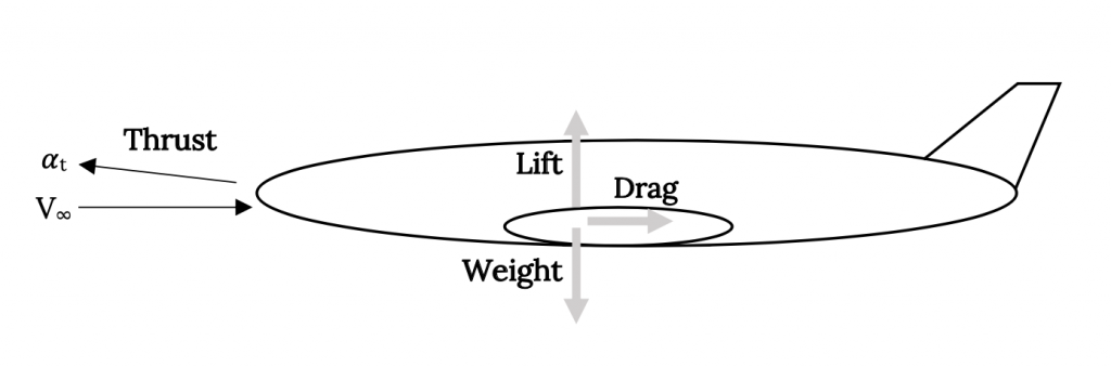
In this text we will consider the very simplest case where the thrust is aligned with the aircraft’s velocity vector. We will also normally assume that the velocity vector is aligned with the direction of flight or flight path. For this most basic case the equations of motion become:
T – D = 0
L – W = 0
Note that this is consistent with the definition of lift and drag as being perpendicular and parallel to the velocity vector or relative wind.
Now we make a simple but very basic assumption that in straight and level flight lift is equal to weight,
L = W
We will use this so often that it will be easy to forget that it does assume that flight is indeed straight and level. Later we will cheat a little and use this in shallow climbs and glides, covering ourselves by assuming “quasi‑straight and level” flight. In the final part of this text we will finally go beyond this assumption when we consider turning flight.
Using the definition of the lift coefficient
and the assumption that lift equals weight, the speed in straight and level flight becomes:
The thrust needed to maintain this speed in straight and level flight is also a function of the aircraft weight. Since T = D and L = W we can write
D/L = T/W
or
Therefore, for straight and level flight we find this relation between thrust and weight:
The above equations for thrust and velocity become our first very basic relations which can be used to ascertain the performance of an aircraft.
4.2 Aerodynamic Stall
Earlier we discussed aerodynamic stall. For an airfoil (2‑D) or wing (3‑D), as the angle of attack is increased a point is reached where the increase in lift coefficient, which accompanies the increase in angle of attack, diminishes. When this occurs the lift coefficient versus angle of attack curve becomes non‑linear as the flow over the upper surface of the wing begins to break away from the surface. This separation of flow may be gradual, usually progressing from the aft edge of the airfoil or wing and moving forward; sudden, as flow breaks away from large portions of the wing at the same time; or some combination of the two. The actual nature of stall will depend on the shape of the airfoil section, the wing planform and the Reynolds number of the flow.
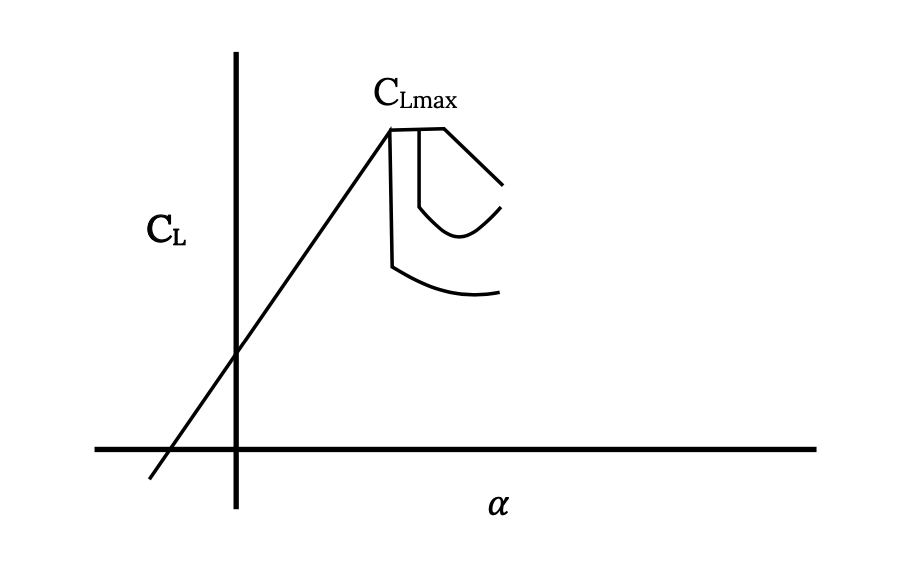
We define the stall angle of attack as the angle where the lift coefficient reaches a maximum, CLmax, and use this value of lift coefficient to calculate a stall speed for straight and level flight.
Note that the stall speed will depend on a number of factors including altitude. If we look at a sea level equivalent stall speed we have
It should be emphasized that stall speed as defined above is based on lift equal to weight or straight and level flight. This is the stall speed quoted in all aircraft operating manuals and used as a reference by pilots. It must be remembered that stall is only a function of angle of attack and can occur at any speed. The definition of stall speed used above results from limiting the flight to straight and level conditions where lift equals weight. This stall speed is not applicable for other flight conditions. For example, in a turn lift will normally exceed weight and stall will occur at a higher flight speed. The same is true in accelerated flight conditions such as climb. For this reason pilots are taught to handle stall in climbing and turning flight as well as in straight and level flight.
For most of this text we will deal with flight which is assumed straight and level and therefore will assume that the straight and level stall speed shown above is relevant. This speed usually represents the lowest practical straight and level flight speed for an aircraft and is thus an important aircraft performance parameter.
We will normally define the stall speed for an aircraft in terms of the maximum gross takeoff weight but it should be noted that the weight of any aircraft will change in flight as fuel is used. For a given altitude, as weight changes the stall speed variation with weight can be found as follows:
It is obvious that as a flight progresses and the aircraft weight decreases, the stall speed also decreases. Since stall speed represents a lower limit of straight and level flight speed it is an indication that an aircraft can usually land at a lower speed than the minimum takeoff speed.
For many large transport aircraft the stall speed of the fully loaded aircraft is too high to allow a safe landing within the same distance as needed for takeoff. In cases where an aircraft must return to its takeoff field for landing due to some emergency situation (such as failure of the landing gear to retract), it must dump or burn off fuel before landing in order to reduce its weight, stall speed and landing speed. Takeoff and landing will be discussed in a later chapter in much more detail.
4.3 Perspectives on Stall
While discussing stall it is worthwhile to consider some of the physical aspects of stall and the many misconceptions that both pilots and the public have concerning stall.
To the aerospace engineer, stall is CLmax, the highest possible lifting capability of the aircraft; but, to most pilots and the public, stall is where the airplane looses all lift! How can it be both? And, if one of these views is wrong, why?
The key to understanding both perspectives of stall is understanding the difference between lift and lift coefficient. Lift is the product of the lift coefficient, the dynamic pressure and the wing planform area. For a given altitude and airplane (wing area) lift then depends on lift coefficient and velocity. It is possible to have a very high lift coefficient CL and a very low lift if velocity is low.
When an airplane is at an angle of attack such that CLmax is reached, the high angle of attack also results in high drag coefficient. The resulting high drag normally leads to a reduction in airspeed which then results in a loss of lift. In a conventionally designed airplane this will be followed by a drop of the nose of the aircraft into a nose down attitude and a loss of altitude as speed is recovered and lift regained. If the pilot tries to hold the nose of the plane up, the airplane will merely drop in a nose up attitude. Pilots are taught to let the nose drop as soon as they sense stall so lift and altitude recovery can begin as rapidly as possible. A good flight instructor will teach a pilot to sense stall at its onset such that recovery can begin before altitude and lift is lost.
It should be noted that if an aircraft has sufficient power or thrust and the high drag present at CLmax can be matched by thrust, flight can be continued into the stall and post‑stall region. This is possible on many fighter aircraft and the post‑stall flight realm offers many interesting possibilities for maneuver in a “dog-fight”.
The general public tends to think of stall as when the airplane drops out of the sky. This can be seen in almost any newspaper report of an airplane accident where the story line will read “the airplane stalled and fell from the sky, nosediving into the ground after the engine failed”. This kind of report has several errors. Stall has nothing to do with engines and an engine loss does not cause stall. Sailplanes can stall without having an engine and every pilot is taught how to fly an airplane to a safe landing when an engine is lost. Stall also doesn’t cause a plane to go into a dive. It is, however, possible for a pilot to panic at the loss of an engine, inadvertently enter a stall, fail to take proper stall recovery actions and perhaps “nosedive” into the ground.
4.4 Drag and Thrust Required
As seen above, for straight and level flight, thrust must be equal to drag. Drag is a function of the drag coefficient CD which is, in turn, a function of a base drag and an induced drag.
CD = CD0 + CDi
We assume that this relationship has a parabolic form and that the induced drag coefficient has the form
CDi = KCL2
We therefore write
CD = CD0 + KCL2
K is found from inviscid aerodynamic theory to be a function of the aspect ratio and planform shape of the wing
where e is unity for an ideal elliptical form of the lift distribution along the wing’s span and less than one for non‑ideal spanwise lift distributions.
The drag coefficient relationship shown above is termed a parabolic drag “polar” because of its mathematical form. It is actually only valid for inviscid wing theory not the whole airplane. In this text we will use this equation as a first approximation to the drag behavior of an entire airplane. While this is only an approximation, it is a fairly good one for an introductory level performance course. It can, however, result in some unrealistic performance estimates when used with some real aircraft data.
The drag of the aircraft is found from the drag coefficient, the dynamic pressure and the wing planform area:
Therefore,
Realizing that for straight and level flight, lift is equal to weight and lift is a function of the wing’s lift coefficient, we can write:
giving:
The above equation is only valid for straight and level flight for an aircraft in incompressible flow with a parabolic drag polar.
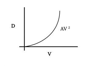
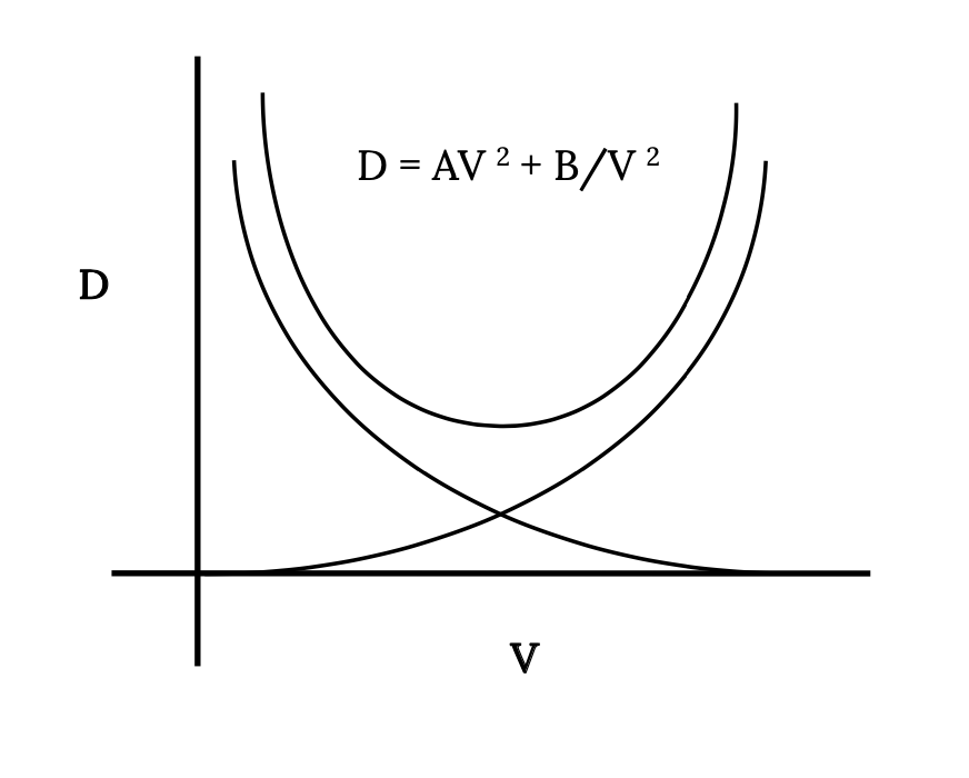
Let’s look at the form of this equation and examine its physical meaning. For a given aircraft at a given altitude most of the terms in the equation are constants and we can write
where
The first term in the equation shows that part of the drag increases with the square of the velocity. This is the base drag term and it is logical that for the basic airplane shape the drag will increase as the dynamic pressure increases. To most observers this is somewhat intuitive.
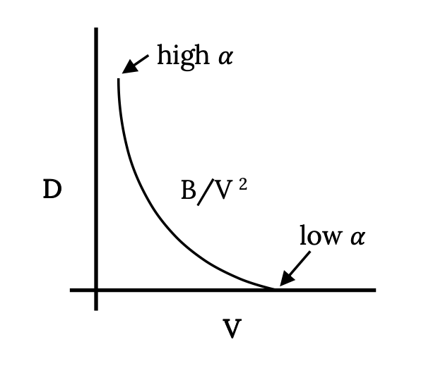
The second term represents a drag which decreases as the square of the velocity increases. It gives an infinite drag at zero speed, however, this is an unreachable limit for normally defined, fixed wing (as opposed to vertical lift) aircraft. It should be noted that this term includes the influence of lift or lift coefficient on drag. The faster an aircraft flies, the lower the value of lift coefficient needed to give a lift equal to weight. Lift coefficient, it is recalled, is a linear function of angle of attack (until stall). If an aircraft is flying straight and level and the pilot maintains level flight while decreasing the speed of the plane, the wing angle of attack must increase in order to provide the lift coefficient and lift needed to equal the weight. As angle of attack increases it is somewhat intuitive that the drag of the wing will increase. As speed is decreased in straight and level flight, this part of the drag will continue to increase exponentially until the stall speed is reached.
Adding the two drag terms together gives the following figure which shows the complete drag variation with velocity for an aircraft with a parabolic drag polar in straight and level flight.
4.5 Minimum Drag
One obvious point of interest on the previous drag plot is the velocity for minimum drag. This can, of course, be found graphically from the plot. We can also take a simple look at the equations to find some other information about conditions for minimum drag.
The requirements for minimum drag are intuitively of interest because it seems that they ought to relate to economy of flight in some way. Later we will find that there are certain performance optima which do depend directly on flight at minimum drag conditions.
At this point we are talking about finding the velocity at which the airplane is flying at minimum drag conditions in straight and level flight. It is important to keep this assumption in mind. We will later find that certain climb and glide optima occur at these same conditions and we will stretch our straight and level assumption to one of “quasi”‑level flight.
We can begin with a very simple look at what our lift, drag, thrust and weight balances for straight and level flight tells us about minimum drag conditions and then we will move on to a more sophisticated look at how the wing shape dependent terms in the drag polar equation (CD0 and K) are related at the minimum drag condition. Ultimately, the most important thing to determine is the speed for flight at minimum drag because the pilot can then use this to fly at minimum drag conditions.
Let’s look at our simple static force relationships:
L = W, T = D
to write
D = W x D/L
which says that minimum drag occurs when the drag divided by lift is a minimum or, inversely, when lift divided by drag is a maximum.
This combination of parameters, L/D, occurs often in looking at aircraft performance. In general, it is usually intuitive that the higher the lift and the lower the drag, the better an airplane. It is not as intuitive that the maximum lift‑to drag ratio occurs at the same flight conditions as minimum drag. This simple analysis, however, shows that
MINIMUM DRAG OCCURS WHEN L/D IS MAXIMUM.
Note that since CL / CD = L/D we can also say that minimum drag occurs when CL/CD is maximum. It is very important to note that minimum drag does not connote minimum drag coefficient.
Minimum drag occurs at a single value of angle of attack where the lift coefficient divided by the drag coefficient is a maximum:
Dmin occurs when (CL/CD)max
As noted above, this is not at the same angle of attack at which CD is at a minimum. It is also not the same angle of attack where lift coefficient is maximum. This should be rather obvious since CLmax occurs at stall and drag is very high at stall.
Since minimum drag is a function only of the ratio of the lift and drag coefficients and not of altitude (density), the actual value of the minimum drag for a given aircraft at a given weight will be invariant with altitude. The actual velocity at which minimum drag occurs is a function of altitude and will generally increase as altitude increases.
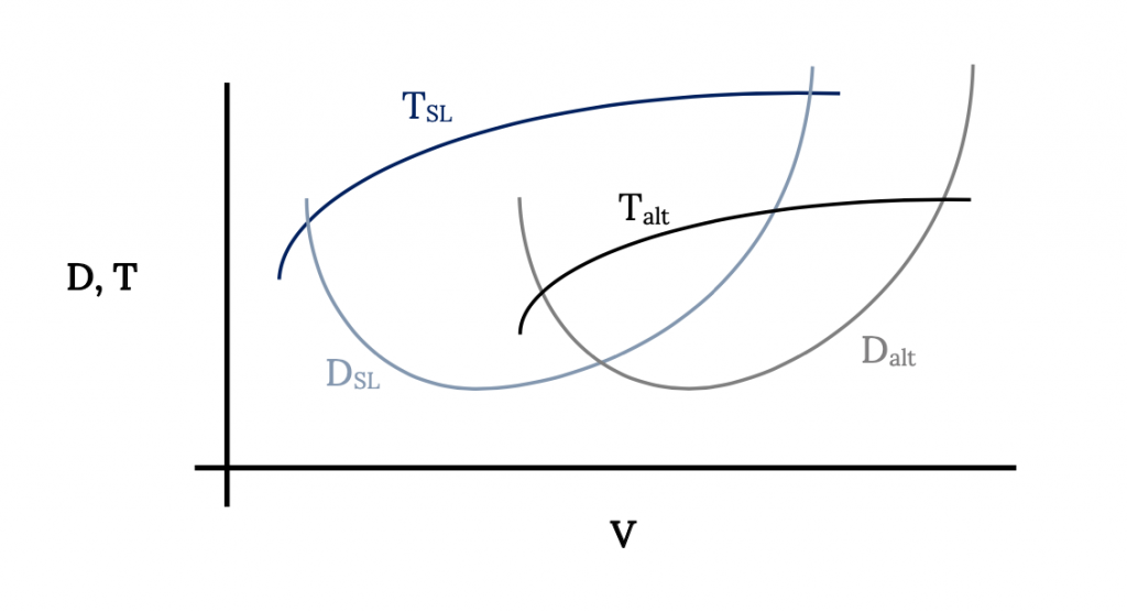
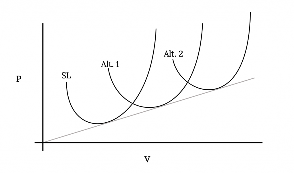
If we assume a parabolic drag polar and plot the drag equation
for drag versus velocity at different altitudes the resulting curves will look somewhat like the following:
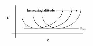
Note that the minimum drag will be the same at every altitude as mentioned earlier and the velocity for minimum drag will increase with altitude.
We discussed in an earlier section the fact that because of the relationship between dynamic pressure at sea level with that at altitude, the aircraft would always perform the same at the same indicated or sea level equivalent airspeed. Indeed, if one writes the drag equation as a function of sea level density and sea level equivalent velocity a single curve will result.
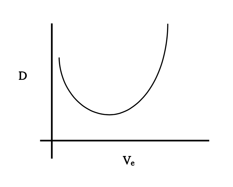
To find the drag versus velocity behavior of an aircraft it is then only necessary to do calculations or plots at sea level conditions and then convert to the true airspeeds for flight at any altitude by using the velocity relationship below.
4.6 Minimum Drag Summary
We know that minimum drag occurs when the lift to drag ratio is at a maximum, but when does that occur; at what value of CL or CD or at what speed?
One way to find CL and CD at minimum drag is to plot one versus the other as shown below. The maximum value of the ratio of lift coefficient to drag coefficient will be where a line from the origin just tangent to the curve touches the curve. At this point are the values of CL and CD for minimum drag. This graphical method of finding the minimum drag parameters works for any aircraft even if it does not have a parabolic drag polar.
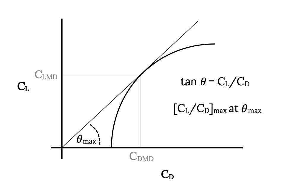
Once CLmd and CDmd are found, the velocity for minimum drag is found from the equation below, provided the aircraft is in straight and level flight
As we already know, the velocity for minimum drag can be found for sea level conditions (the sea level equivalent velocity) and from that it is easy to find the minimum drag speed at altitude.
It should also be noted that when the lift and drag coefficients for minimum drag are known and the weight of the aircraft is known the minimum drag itself can be found from
It is common to assume that the relationship between drag and lift is the one we found earlier, the so called parabolic drag polar. For the parabolic drag polar
it is easy to take the derivative with respect to the lift coefficient and set it equal to zero to determine the conditions for the minimum ratio of drag coefficient to lift coefficient, which was a condition for minimum drag.
Hence,
This gives
or
and
The above is the condition required for minimum drag with a parabolic drag polar.
Now, we return to the drag polar
and for minimum drag we can write
which, with the above, gives
or
From this we can find the value of the maximum lift‑to‑drag ratio in terms of basic drag parameters
And the speed at which this occurs in straight and level flight is
So we can write the minimum drag velocity as
or the sea level equivalent minimum drag speed as
4.7 Review: Minimum Drag Conditions for a Parabolic Drag Polar
At this point we know a lot about minimum drag conditions for an aircraft with a parabolic drag polar in straight and level flight. The following equations may be useful in the solution of many different performance problems to be considered later in this text. There will be several flight conditions which will be found to be optimized when flown at minimum drag conditions. It is therefore suggested that the student write the following equations on a separate page in her or his class notes for easy reference.
EXAMPLE 4.1
An aircraft which weighs 3000 pounds has a wing area of 175 square feet and an aspect ratio of seven with a wing aerodynamic efficiency factor (e) of 0.95. If the base drag coefficient, CDO, is 0.028, find the minimum drag at sea level and at 10,000 feet altitude, the maximum lift‑to-drag ratio and the values of lift and drag coefficient for minimum drag. Also find the velocities for minimum drag in straight and level flight at both sea level and 10,000 feet. We need to first find the term K in the drag equation.
K = 1 / (πARe) = 0.048
Now we can find
We can check this with
The velocity for minimum drag is the first of these that depends on altitude.
At sea level
To find the velocity for minimum drag at 10,000 feet we an recalculate using the density at that altitude or we can use
It is suggested that at this point the student use the drag equation
and make graphs of drag versus velocity for both sea level and 10,000 foot altitude conditions, plotting drag values at 20 fps increments. The plots would confirm the above values of minimum drag velocity and minimum drag.
4.8 Flying at Minimum Drag
One question which should be asked at this point but is usually not answered in a text on aircraft performance is “Just how the heck does the pilot make that airplane fly at minimum drag conditions anyway?”
The answer, quite simply, is to fly at the sea level equivalent speed for minimum drag conditions. The pilot sets up or “trims” the aircraft to fly at constant altitude (straight and level) at the indicated airspeed (sea level equivalent speed) for minimum drag as given in the aircraft operations manual. All the pilot need do is hold the speed and altitude constant.
4.9 Drag in Compressible Flow
For the purposes of an introductory course in aircraft performance we have limited ourselves to the discussion of lower speed aircraft; ie, airplanes operating in incompressible flow. As discussed earlier, analytically, this would restrict us to consideration of flight speeds of Mach 0.3 or less (less than 300 fps at sea level), however, physical realities of the onset of drag rise due to compressibility effects allow us to extend our use of the incompressible theory to Mach numbers of around 0.6 to 0.7. This is the range of Mach number where supersonic flow over places such as the upper surface of the wing has reached the magnitude that shock waves may occur during flow deceleration resulting in energy losses through the shock and in drag rises due to shock‑induced flow separation over the wing surface. This drag rise was discussed in Chapter 3.
As speeds rise to the region where compressiblility effects must be considered we must take into account the speed of sound a and the ratio of specific heats of air, gamma.
Gamma for air at normal lower atmospheric temperatures has a value of 1.4.
Starting again with the relation for a parabolic drag polar, we can multiply and divide by the speed of sound to rewrite the relation in terms of Mach number.
where
or
The resulting equation above is very similar in form to the original drag polar relation and can be used in a similar fashion. For example, to find the Mach number for minimum drag in straight and level flight we would take the derivative with respect to Mach number and set the result equal to zero. The complication is that some terms which we considered constant under incompressible conditions such as K and CDO may now be functions of Mach number and must be so evaluated.
Often the equation above must be solved itteratively.
4.10 Review
To this point we have examined the drag of an aircraft based primarily on a simple model using a parabolic drag representation in incompressible flow. We have further restricted our analysis to straight and level flight where lift is equal to weight and thrust equals drag.
The aircraft can fly straight and level at a wide range of speeds, provided there is sufficient power or thrust to equal or overcome the drag at those speeds. The student needs to understand the physical aspects of this flight.
We looked at the speed for straight and level flight at minimum drag conditions. One could, of course, always cruise at that speed and it might, in fact, be a very economical way to fly (we will examine this later in a discussion of range and endurance). However, since “time is money” there may be reason to cruise at higher speeds. It also might just be more fun to fly faster. Flight at higher than minimum-drag speeds will require less angle of attack to produce the needed lift (to equal weight) and the upper speed limit will be determined by the maximum thrust or power available from the engine.
Cruise at lower than minimum drag speeds may be desired when flying approaches to landing or when flying in holding patterns or when flying other special purpose missions. This will require a higher than minimum-drag angle of attack and the use of more thrust or power to overcome the resulting increase in drag. The lower limit in speed could then be the result of the drag reaching the magnitude of the power or the thrust available from the engine; however, it will normally result from the angle of attack reaching the stall angle. Hence, stall speed normally represents the lower limit on straight and level cruise speed.
It must be remembered that all of the preceding is based on an assumption of straight and level flight. If an aircraft is flying straight and level at a given speed and power or thrust is added, the plane will initially both accelerate and climb until a new straight and level equilibrium is reached at a higher altitude. The pilot can control this addition of energy by changing the plane’s attitude (angle of attack) to direct the added energy into the desired combination of speed increase and/or altitude increase. If the engine output is decreased, one would normally expect a decrease in altitude and/or speed, depending on pilot control input.
We must now add the factor of engine output, either thrust or power, to our consideration of performance. It is normal to refer to the output of a jet engine as thrust and of a propeller engine as power. We will first consider the simpler of the two cases, thrust.
4.11 Thrust
We have said that for an aircraft in straight and level flight, thrust must equal drag. If the thrust of the aircraft’s engine exceeds the drag for straight and level flight at a given speed, the airplane will either climb or accelerate or do both. It could also be used to make turns or other maneuvers. The drag encountered in straight and level flight could therefore be called the thrust required (for straight and level flight). The thrust actually produced by the engine will be referred to as the thrust available.
Although we can speak of the output of any aircraft engine in terms of thrust, it is conventional to refer to the thrust of jet engines and the power of prop engines. A propeller, of course, produces thrust just as does the flow from a jet engine; however, for an engine powering a propeller (either piston or turbine), the output of the engine itself is power to a shaft. Thus when speaking of such a propulsion system most references are to its power. When speaking of the propeller itself, thrust terminology may be used.
The units employed for discussions of thrust are Newtons in the SI system and pounds in the English system. Since the English units of pounds are still almost universally used when speaking of thrust, they will normally be used here.
Thrust is a function of many variables including efficiencies in various parts of the engine, throttle setting, altitude, Mach number and velocity. A complete study of engine thrust will be left to a later propulsion course. For our purposes very simple models of thrust will suffice with assumptions that thrust varies with density (altitude) and throttle setting and possibly, velocity. We already found one such relationship in Chapter two with the momentum equation. Often we will simplify things even further and assume that thrust is invariant with velocity for a simple jet engine.
If we know the thrust variation with velocity and altitude for a given aircraft we can add the engine thrust curves to the drag curves for straight and level flight for that aircraft as shown below. We will normally assume that since we are interested in the limits of performance for the aircraft we are only interested in the case of 100% throttle setting. It is obvious that other throttle settings will give thrusts at any point below the 100% curves for thrust.
In the figure above it should be noted that, although the terminology used is thrust and drag, it may be more meaningful to call these curves thrust available and thrust required when referring to the engine output and the aircraft drag, respectively.
4.12 Minimum and Maximum Speeds
The intersections of the thrust and drag curves in the figure above obviously represent the minimum and maximum flight speeds in straight and level flight. Above the maximum speed there is insufficient thrust available from the engine to overcome the drag (thrust required) of the aircraft at those speeds. The same is true below the lower speed intersection of the two curves.
The true lower speed limitation for the aircraft is usually imposed by stall rather than the intersection of the thrust and drag curves. Stall speed may be added to the graph as shown below:
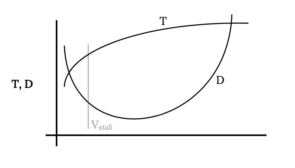
The area between the thrust available and the drag or thrust required curves can be called the flight envelope. The aircraft can fly straight and level at any speed between these upper and lower speed intersection points. Between these speed limits there is excess thrust available which can be used for flight other than straight and level flight. This excess thrust can be used to climb or turn or maneuver in other ways. We will look at some of these maneuvers in a later chapter. For now we will limit our investigation to the realm of straight and level flight.
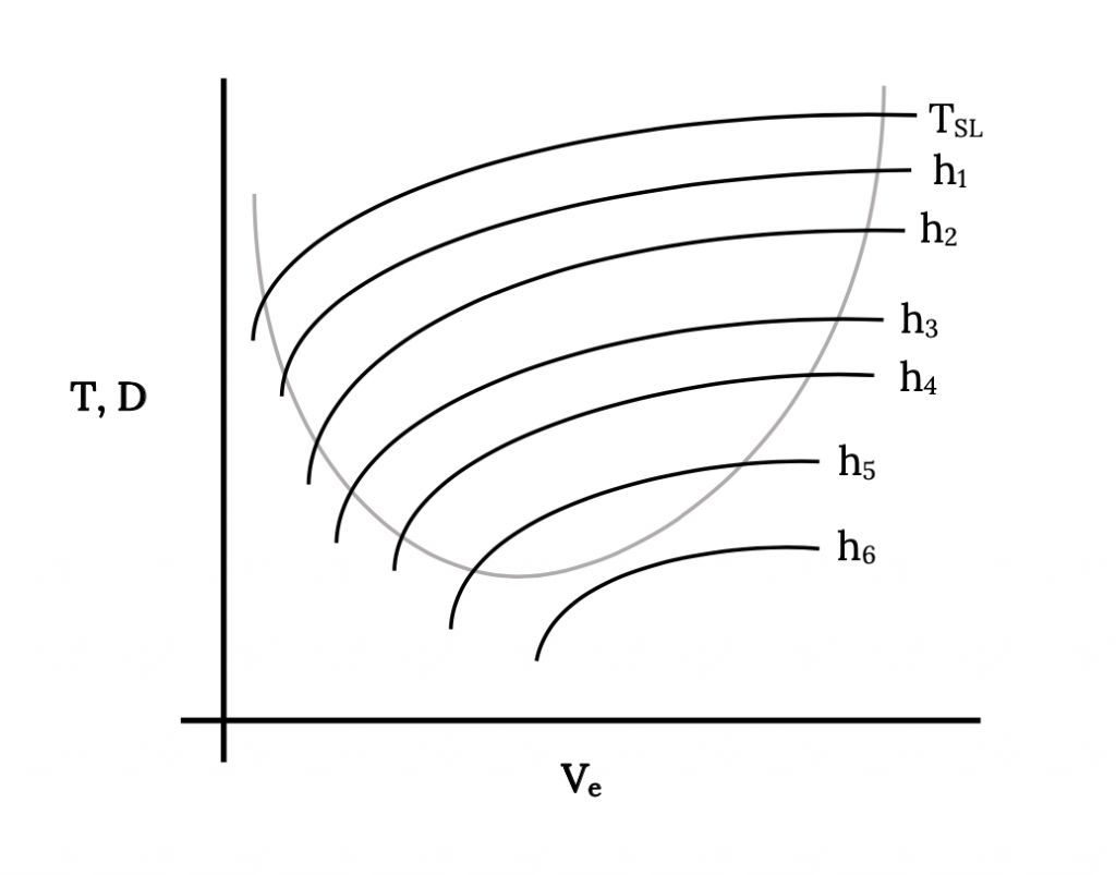
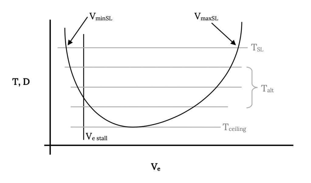
Note that at the higher altitude, the decrease in thrust available has reduced the “flight envelope”, bringing the upper and lower speed limits closer together and reducing the excess thrust between the curves. As thrust is continually reduced with increasing altitude, the flight envelope will continue to shrink until the upper and lower speeds become equal and the two curves just touch. This can be seen more clearly in the figure below where all data is plotted in terms of sea level equivalent velocity. In the example shown, the thrust available at h6 falls entirely below the drag or thrust required curve. This means that the aircraft can not fly straight and level at that altitude. That altitude is said to be above the “ceiling” for the aircraft. At some altitude between h5 and h6 feet there will be a thrust available curve which will just touch the drag curve. That altitude will be the ceiling altitude of the airplane, the altitude at which the plane can only fly at a single speed. We will have more to say about ceiling definitions in a later section.
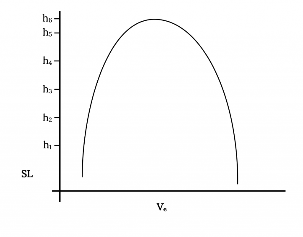
Another way to look at these same speed and altitude limits is to plot the intersections of the thrust and drag curves on the above figure against altitude as shown below. This shows another version of a flight envelope in terms of altitude and velocity. This type of plot is more meaningful to the pilot and to the flight test engineer since speed and altitude are two parameters shown on the standard aircraft instruments and thrust is not.
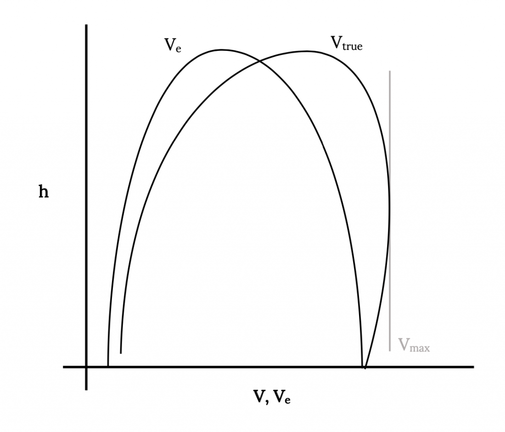
It may also be meaningful to add to the figure above a plot of the same data using actual airspeed rather than the indicated or sea level equivalent airspeeds. This can be done rather simply by using the square root of the density ratio (sea level to altitude) as discussed earlier to convert the equivalent speeds to actual speeds. This is shown on the graph below. Note that at sea level V = Ve and also there will be some altitude where there is a maximum true airspeed.
4.13 Special Case of Constant Thrust
A very simple model is often employed for thrust from a jet engine. The assumption is made that thrust is constant at a given altitude. We will use this assumption as our standard model for all jet aircraft unless otherwise noted in examples or problems. Later we will discuss models for variation of thrust with altitude.
The above model (constant thrust at altitude) obviously makes it possible to find a rather simple analytical solution for the intersections of the thrust available and drag (thrust required) curves. We will let thrust equal a constant
T = T0
therefore, in straight and level flight where thrust equals drag, we can write
where q is a commonly used abbreviation for the dynamic pressure.
or
and rearranging as a quadratic equation
Solving the above equation gives
or
In terms of the sea level equivalent speed
These solutions are, of course, double valued. The higher velocity is the maximum straight and level flight speed at the altitude under consideration and the lower solution is the nominal minimum straight and level flight speed (the stall speed will probably be a higher speed, representing the true minimum flight speed).
There are, of course, other ways to solve for the intersection of the thrust and drag curves. Sometimes it is convenient to solve the equations for the lift coefficients at the minimum and maximum speeds. To set up such a solution we first return to the basic straight and level flight equations T = T0 = D and L = W.
or
solving for CL
This solution will give two values of the lift coefficient. The larger of the two values represents the minimum flight speed for straight and level flight while the smaller CL is for the maximum flight speed. The matching speed is found from the relation
4.14 Review for Constant Thrust
The figure below shows graphically the case discussed above. From the solution of the thrust equals drag relation we obtain two values of either lift coefficient or speed, one for the maximum straight and level flight speed at the chosen altitude and the other for the minimum flight speed. The stall speed will probably exceed the minimum straight and level flight speed found from the thrust equals drag solution, making it the true minimum flight speed.
As altitude increases T0 will normally decrease and VMIN and VMAX will move together until at a ceiling altitude they merge to become a single point.
It is normally assumed that the thrust of a jet engine will vary with altitude in direct proportion to the variation in density. This assumption is supported by the thrust equations for a jet engine as they are derived from the momentum equations introduced in chapter two of this text. We can therefore write:
EXAMPLE 4.2
Earlier in this chapter we looked at a 3000 pound aircraft with a 175 square foot wing area, aspect ratio of seven and CDO of 0.028 with e = 0.95. Let us say that the aircraft is fitted with a small jet engine which has a constant thrust at sea level of 400 pounds. Find the maximum and minimum straight and level flight speeds for this aircraft at sea level and at 10,000 feet assuming that thrust available varies proportionally to density.
If, as earlier suggested, the student, plotted the drag curves for this aircraft, a graphical solution is simple. One need only add a straight line representing 400 pounds to the sea level plot and the intersections of this line with the sea level drag curve give the answer. The same can be done with the 10,000 foot altitude data, using a constant thrust reduced in proportion to the density.
Given a standard atmosphere density of 0.001756 sl/ft3, the thrust at 10,000 feet will be 0.739 times the sea level thrust or 296 pounds. Using the two values of thrust available we can solve for the velocity limits at sea level and at l0,000 ft.
= 63053 or 5661
VSL = 251 ft/sec (max)
or = 75 ft/sec (min)
Thus the equation gives maximum and minimum straight and level flight speeds as 251 and 75 feet per second respectively.
It is suggested that the student do similar calculations for the 10,000 foot altitude case. Note that one cannot simply take the sea level velocity solutions above and convert them to velocities at altitude by using the square root of the density ratio. The equations must be solved again using the new thrust at altitude. The student should also compare the analytical solution results with the graphical results.
As mentioned earlier, the stall speed is usually the actual minimum flight speed. If the maximum lift coefficient has a value of 1.2, find the stall speeds at sea level and add them to your graphs.
4.15 Performance in Terms of Power
The engine output of all propeller powered aircraft is expressed in terms of power. Power is really energy per unit time. While the propeller output itself may be expressed as thrust if desired, it is common to also express it in terms of power.
While at first glance it may seem that power and thrust are very different parameters, they are related in a very simple manner through velocity. Power is thrust multiplied by velocity. The units for power are Newton‑meters per second or watts in the SI system and horsepower in the English system. As before, we will use primarily the English system. The reason is rather obvious. The author challenges anyone to find any pilot, mechanic or even any automobile driver anywhere in the world who can state the power rating for their engine in watts! Watts are for light bulbs: horsepower is for engines!
Actually, our equations will result in English system power units of foot‑pounds per second. The conversion is
one HP = 550 foot-pounds/second.
We will speak of two types of power; power available and power required. Power required is the power needed to overcome the drag of the aircraft
Preq = D x V
Power available is equal to the thrust multiplied by the velocity.
Pav = T x V
It should be noted that we can start with power and find thrust by dividing by velocity, or we can multiply thrust by velocity to find power. There is no reason for not talking about the thrust of a propeller propulsion system or about the power of a jet engine. The use of power for propeller systems and thrust for jets merely follows convention and also recognizes that for a jet, thrust is relatively constant with speed and for a prop, power is relatively invariant with speed.
Power available is the power which can be obtained from the propeller. Recognizing that there are losses between the engine and propeller we will distinguish between power available and shaft horsepower. Shaft horsepower is the power transmitted through the crank or drive shaft to the propeller from the engine. The engine may be piston or turbine or even electric or steam. The propeller turns this shaft power (Ps) into propulsive power with a certain propulsive efficiency, ηp.
The propulsive efficiency is a function of propeller speed, flight speed, propeller design and other factors.
It is obvious that both power available and power required are functions of speed, both because of the velocity term in the relation and from the variation of both drag and thrust with speed. For the ideal jet engine which we assume to have a constant thrust, the variation in power available is simply a linear increase with speed.
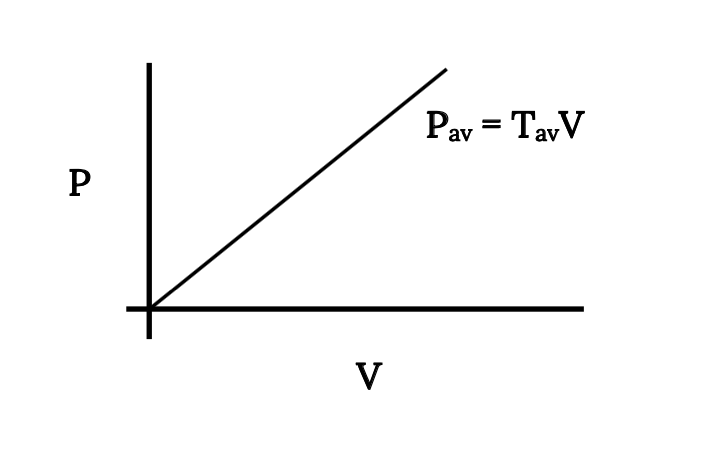
It is interesting that if we are working with a jet where thrust is constant with respect to speed, the equations above give zero power at zero speed. This is not intuitive but is nonetheless true and will have interesting consequences when we later examine rates of climb.
Another consequence of this relationship between thrust and power is that if power is assumed constant with respect to speed (as we will do for prop aircraft) thrust becomes infinite as speed approaches zero. This means that a Cessna 152 when standing still with the engine running has infinitely more thrust than a Boeing 747 with engines running full blast. It also has more power! What an ego boost for the private pilot!
In using the concept of power to examine aircraft performance we will do much the same thing as we did using thrust. We will speak of the intersection of the power required and power available curves determining the maximum and minimum speeds. We will find the speed for minimum power required. We will look at the variation of these with altitude. The graphs we plot will look like that below.
While the maximum and minimum straight and level flight speeds we determine from the power curves will be identical to those found from the thrust data, there will be some differences. One difference can be noted from the figure above. Unlike minimum drag, which was the same magnitude at every altitude, minimum power will be different at every altitude. This means it will be more complicated to collapse the data at all altitudes into a single curve.
4.16 Power Required
The power required plot will look very similar to that seen earlier for thrust required (drag). It is simply the drag multiplied by the velocity. If we continue to assume a parabolic drag polar with constant values of CDO and K we have the following relationship for power required:
We can plot this for given values of CDO, K, W and S (for a given aircraft) for various altitudes as shown in the following example.
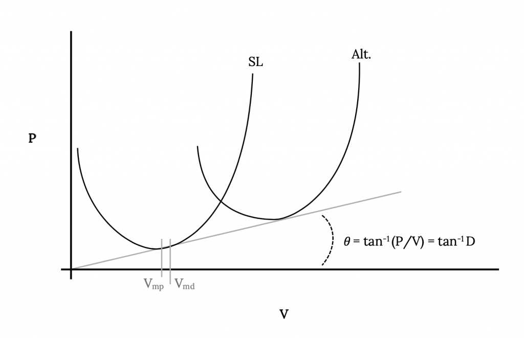
We will note that the minimum values of power will not be the same at each altitude. Recalling that the minimum values of drag were the same at all altitudes and that power required is drag times velocity, it is logical that the minimum value of power increases linearly with velocity. We should be able to draw a straight line from the origin through the minimum power required points at each altitude.
The minimum power required in straight and level flight can, of course be taken from plots like the one above. We would also like to determine the values of lift and drag coefficient which result in minimum power required just as we did for minimum drag.
One might assume at first that minimum power for a given aircraft occurs at the same conditions as those for minimum drag. This is, of course, not true because of the added dependency of power on velocity. We can begin to understand the parameters which influence minimum required power by again returning to our simple force balance equations for straight and level flight:
Thus, for a given aircraft (weight and wing area) and altitude (density) the minimum required power for straight and level flight occurs when the drag coefficient divided by the lift coefficient to the two‑thirds power is at a minimum.
Assuming a parabolic drag polar, we can write an equation for the above ratio of coefficients and take its derivative with respect to the lift coefficient (since CL is linear with angle of attack this is the same as looking for a maximum over the range of angle of attack) and set it equal to zero to find a maximum.
Note that
The lift coefficient for minimum required power is higher (1.732 times) than that for minimum drag conditions.
Knowing the lift coefficient for minimum required power it is easy to find the speed at which this will occur.
Note that the velocity for minimum required power is lower than that for minimum drag.
The minimum power required and minimum drag velocities can both be found graphically from the power required plot. Minimum power is obviously at the bottom of the curve. Realizing that drag is power divided by velocity and that a line drawn from the origin to any point on the power curve is at an angle to the velocity axis whose tangent is power divided by velocity, then the line which touches the curve with the smallest angle must touch it at the minimum drag condition. From this we can graphically determine the power and velocity at minimum drag and then divide the former by the latter to get the minimum drag. Note that this graphical method works even for nonparabolic drag cases. Since we know that all altitudes give the same minimum drag, all power required curves for the various altitudes will be tangent to this same line with the point of tangency being the minimum drag point.
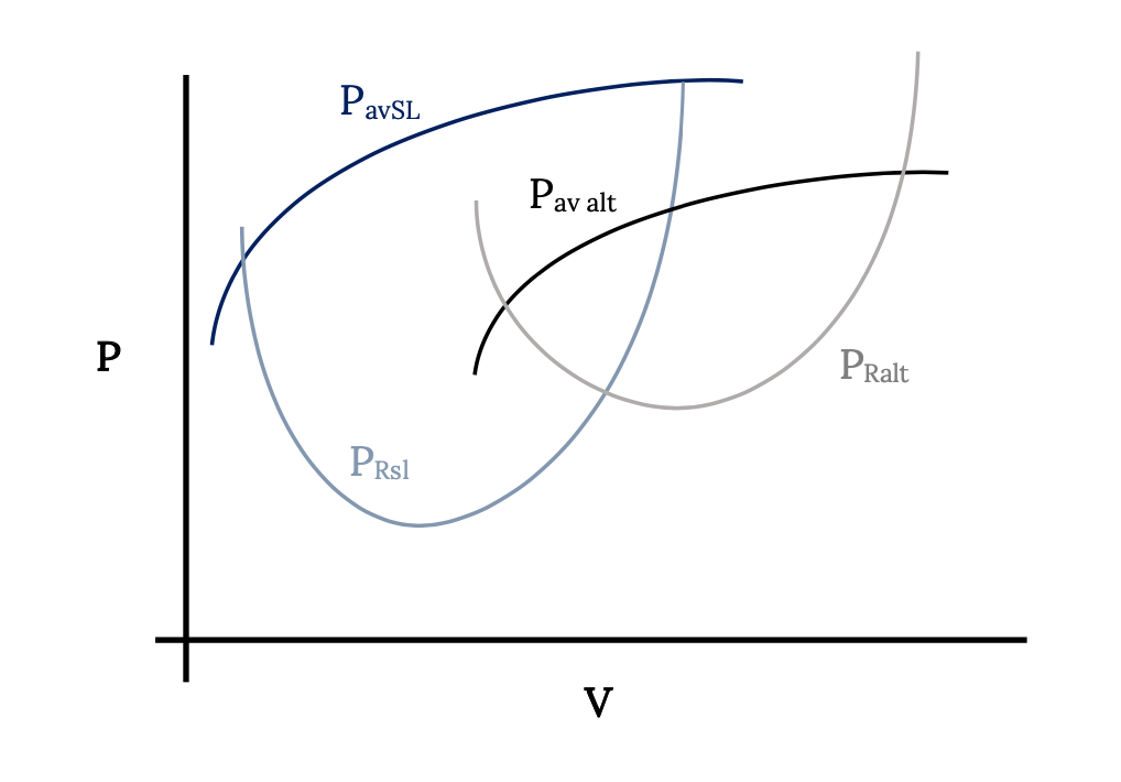
One further item to consider in looking at the graphical representation of power required is the condition needed to collapse the data for all altitudes to a single curve. In the case of the thrust required or drag this was accomplished by merely plotting the drag in terms of sea level equivalent velocity. That will not work in this case since the power required curve for each altitude has a different minimum. Plotting all data in terms of Ve would compress the curves with respect to velocity but not with respect to power. The result would be a plot like the following:
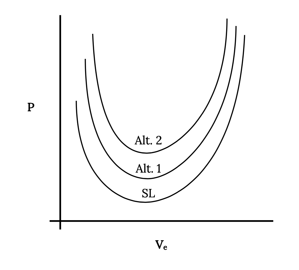
Knowing that power required is drag times velocity we can relate the power required at sea level to that at any altitude.
or
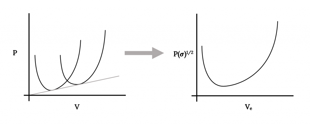
The result is that in order to collapse all power required data to a single curve we must plot power multiplied by the square root of sigma versus sea level equivalent velocity. This, therefore, will be our convention in plotting power data.
4.17 Review
In the preceding we found the following equations for the determination of minimum power required conditions:
We can also write
Thus, the drag coefficient for minimum power required conditions is twice that for minimum drag. We also can write
Since minimum power required conditions are important and will be used later to find other performance parameters it is suggested that the student write the above relationships on a special page in his or her notes for easy reference.
Later we will take a complete look at dealing with the power available. If we know the power available we can, of course, write an equation with power required equated to power available and solve for the maximum and minimum straight and level flight speeds much as we did with the thrust equations. The power equations are, however not as simple as the thrust equations because of their dependence on the cube of the velocity. Often the best solution is an itterative one.
If the power available from an engine is constant (as is usually assumed for a prop engine) the relation equating power available and power required is
For a jet engine where the thrust is modeled as a constant the equation reduces to that used in the earlier section on Thrust based performance calculations.
EXAMPLE 4.3
For the same 3000 lb airplane used in earlier examples calculate the velocity for minimum power.
- It is suggested that the student make plots of the power required for straight and level flight at sea level and at 10,000 feet altitude and graphically verify the above calculated values.
- It is also suggested that from these plots the student find the speeds for minimum drag and compare them with those found earlier.
4.18 Summary
This chapter has looked at several elements of performance in straight and level flight. A simple model for drag variation with velocity was proposed (the parabolic drag polar) and this was used to develop equations for the calculations of minimum drag flight conditions and to find maximum and minimum flight speeds at various altitudes. Graphical methods were also stressed and it should be noted again that these graphical methods will work regardless of the drag model used.
It is strongly suggested that the student get into the habit of sketching a graph of the thrust and or power versus velocity curves as a visualization aid for every problem, even if the solution used is entirely analytical. Such sketches can be a valuable tool in developing a physical feel for the problem and its solution.
Homework 4
1. Use the momentum theorem to find the thrust for a jet engine where the following conditions are known:
| inlet velocity | 300 fps |
| inlet density | 0.0023 sl/ft^3 |
| inlet area | 4 ft^2 |
| exit velocity | 1800 fps |
| exit density | unknown |
| exit area | 2 ft^2 |
| fuel flow rate | 5 lbm/sec |
Assume steady flow and that the inlet and exit pressures are atmospheric.
2. We found that the thrust from a propeller could be described by the equation T = T0 – aV2. Based on this equation, describe how you would set up a simple wind tunnel experiment to determine values for T0 and a for a model airplane engine. Assume you have access to a wind tunnel, a pitot-static tube, a u-tube manometer, and a load cell which will measure thrust. Draw a sketch of your experiment.
References
Figure 4.1: Kindred Grey (2021). “Static Force Balance in Straight and Level Flight.” CC BY 4.0. Adapted from James F. Marchman (2004). CC BY 4.0. Available from https://archive.org/details/4.1_20210804
Figure 4.2: Kindred Grey (2021). “Different Types of Stall.” CC BY 4.0. Adapted from James F. Marchman (2004). CC BY 4.0. Available from https://archive.org/details/4.2_20210804
Figure 4.3: Kindred Grey (2021). “Part of Drag Increases With Velocity Squared.” CC BY 4.0. Adapted from James F. Marchman (2004). CC BY 4.0. Available from https://archive.org/details/4.3_20210804
Figure 4.4: Kindred Grey (2021). “Part of Drag Decreases With Velocity Squared.” CC BY 4.0. Adapted from James F. Marchman (2004). CC BY 4.0. Available from https://archive.org/details/4.4_20210804
Figure 4.5: Kindred Grey (2021). “Total Drag Variation With Velocity.” CC BY 4.0. Adapted from James F. Marchman (2004). CC BY 4.0. Available from https://archive.org/details/4.5_20210804
Figure 4.6: Kindred Grey (2021). “Altitude Effect on Drag Variation.” CC BY 4.0. Adapted from James F. Marchman (2004). CC BY 4.0. Retrieved from https://archive.org/details/4.6_20210804
Figure 4.7: Kindred Grey (2021). “Drag Versus Sea Level Equivalent (Indicated) Velocity.” CC BY 4.0. Adapted from James F. Marchman (2004). CC BY 4.0. Available from https://archive.org/details/4.7_20210804
Figure 4.8: Kindred Grey (2021). “Graphical Method for Determining Minimum Drag Conditions.” CC BY 4.0. Adapted from James F. Marchman (2004). CC BY 4.0. Available from https://archive.org/details/4.8_20210805
Figure 4.9: Kindred Grey (2021). “Thrust and Drag Variation With Velocity.” CC BY 4.0. Adapted from James F. Marchman (2004). CC BY 4.0. Available from https://archive.org/details/4.9_20210805
Figure 4.10: Kindred Grey (2021). “Minimum and Maximum Speeds for Straight & Level Flight.” CC BY 4.0. Adapted from James F. Marchman (2004). CC BY 4.0. Available from https://archive.org/details/4.10_20210805
Figure 4.11: Kindred Grey (2021). “Thrust Variation With Altitude vs Sea Level Equivalent Speed.” CC BY 4.0. Adapted from James F. Marchman (2004). CC BY 4.0. Available from https://archive.org/details/4.11_20210805
Figure 4.12: Kindred Grey (2021). “Straight & Level Flight Speed Envelope With Altitude.” CC BY 4.0. Adapted from James F. Marchman (2004). CC BY 4.0. Available from https://archive.org/details/4.12_20210805
Figure 4.13: Kindred Grey (2021). “True Maximum Airspeed Versus Altitude .” CC BY 4.0. Adapted from James F. Marchman (2004). CC BY 4.0. Available from https://archive.org/details/4.13_20210805
Figure 4.14: Kindred Grey (2021). “Graphical Solution for Constant Thrust at Each Altitude .” CC BY 4.0. Adapted from James F. Marchman (2004). CC BY 4.0. Available from https://archive.org/details/4.14_20210805
Figure 4.15: Kindred Grey (2021). “Power Available Varies Linearly With Velocity.” CC BY 4.0. Adapted from James F. Marchman (2004). CC BY 4.0. Available from https://archive.org/details/4.15_20210805
Figure 4.16: Kindred Grey (2021). “Power Required and Available Variation With Altitude.” CC BY 4.0. Adapted from James F. Marchman (2004). CC BY 4.0. Available from https://archive.org/details/4.16_20210805
Figure 4.17: Kindred Grey (2021). “Power Required Variation With Altitude.” CC BY 4.0. Adapted from James F. Marchman (2004). CC BY 4.0. Available from https://archive.org/details/4.17_20210805
Figure 4.18: Kindred Grey (2021). “Graphical Determination of Minimum Drag and Minimum Power Speeds.” CC BY 4.0. Adapted from James F. Marchman (2004). CC BY 4.0. Available from https://archive.org/details/4.18_20210805
Figure 4.19: Kindred Grey (2021). “Plot of Power Required vs Sea Level Equivalent Speed.” CC BY 4.0. Adapted from James F. Marchman (2004). CC BY 4.0. Available from https://archive.org/details/4.19_20210805
Figure 4.20: Kindred Grey (2021). “Compression of Power Data to a Single Curve.” CC BY 4.0. Adapted from James F. Marchman (2004). CC BY 4.0. Available from https://archive.org/details/4.20_20210805
