Chapter 3. Additional Aerodynamics Tools
Introduction
All of the introductory aerodynamic concepts needed for the aircraft performance material to be covered in the following chapters were presented in Chapter 1. In general, it will be left up to the readers’ choice of many excellent texts on the subject of aerodynamics to provide in-depth coverage of the field, including complete derivations of aerodynamic theories and discussions of their usage. The field of aerodynamics is often separated into five or more segments based on the flow characteristics and the assumptions that can or must be made to analyze those flows in detail. These divisions would normally include:
- Incompressible or subsonic aerodynamics
- Transonic aerodynamics
- Supersonic aerodynamics
- Hypersonic aerodynamics
- Boundary layer theory
Other, even more specialized, segments of the aerodynamics field might include such topics as rarefied gas dynamics and magneto-hydrodynamics.
In chapter one we looked at a few basic concepts relevant to the first three topics above with an emphasis on the incompressible flow regime and, hopefully, enough discussion of the assumptions involved for the reader to recognize when he or she is in danger of the need to account for transonic or supersonic flow effects. We looked at some of the basic conclusions that come from an analysis of two and three dimensional flow around airfoils and wings. We learned, for example, that the camber of an airfoil will determine the angle of attack at which the airfoil lift coefficient is zero and that we can temporarily change camber with things like wing warping or its modern equivalent, “morphing”, or, in a more conventional manner with flaps. We might be curious as to how much of a change camber can give in the zero lift angle of attack.
We learned that there is a certain type of spanwise lift distribution on a three dimensional wing that will give “optimum” aerodynamic performance by giving “minimum induced drag” and we found that higher aspect ratio wing planforms also give better performance than wings with low AR.
In this chapter we are going to take a very elementary look at these two fundamental wing and airfoil configuration effects, just enough of a look so we will have at least one or two basic tools that might help us find out something about the effects of wing design on aircraft performance should we need to do so. We will do this, not through the type of thorough analysis that would be found in most good aerodynamic textbooks, but with a couple of somewhat over simplified approaches that are, nonetheless, often useful.
In order to develop the desired “back of the envelope” methods of looking at some basic influences of airfoil and wing shape on aerodynamics and performance we need to first take a quick look at how an aerodynamicist would make a mathematical model of a wing or airfoil. Let’s begin by looking at the flow around a lifting airfoil.
3.1 Airfoils (2-D Aerodynamics)
For an airfoil or wing to product lift the flow over its upper surface must move faster than the flow over its lower surface. If this occurs, Bernoulli’s equation would tell us that the faster flow over the upper surface will give a lower pressure than the slower flow over the lower surface and this pressure differential will produce lift. If we look at the flow at a point some distance behind the leading edge of an airfoil we will find that we could represent it somewhat as shown in the figure below with a large velocity vector on top of the airfoil and a smaller one on the bottom.
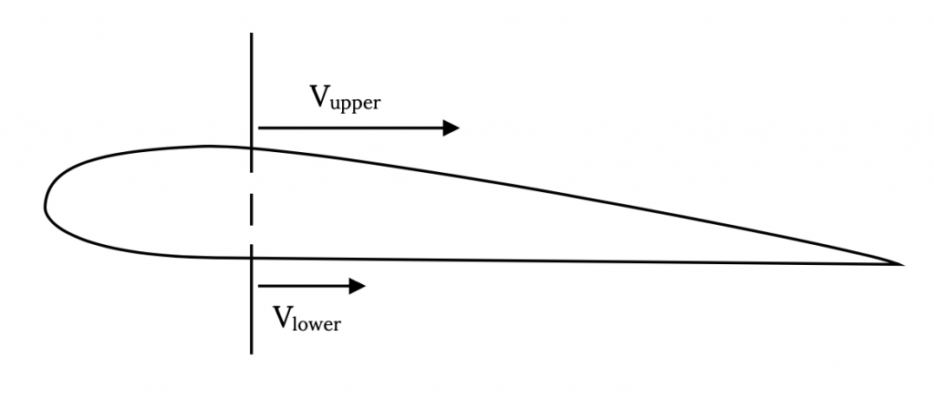
Another way to represent this same flow would be with a combination of a “uniform” flow and a circular flow, such that the velocities add on top of the wing and subtract on the bottom as shown below.
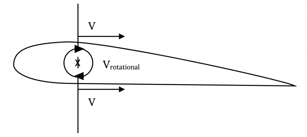
If these two flows can be said to end up giving the same result, the flow shown in Figure 3.2 can be said to be a way to model the flow around an airfoil. This, in fact, works very well and is the basic idea behind the way an aerodynamicist would model the flow around an airfoil.
We could look at the upper and lower surface velocities at several points along the chord and find that at any point we can model that local flow by a “uniform” flow and a circular type flow as shown in Figure 3.3.
In this model, the “uniform” flows on the upper and lower surface would be exactly the same as the upstream or “freestream” velocity, V∞. The only thing that would change at each position along the chord line would be the circular type flow, which would get more powerful where the speed differential between upper and lower surfaces gets larger and less as it gets smaller.
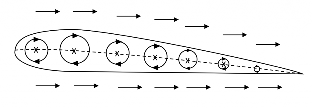
These “circular” flows are known as vortices (a single circular flow is a vortex) and they are the mathematical equivalent of a little tornado. It turns out that vortices are very important flows in aerodynamics and they occur physically in many places. Of course, there are no vortices in the middle of a wing. Here, we are just using a real physical flow, a vortex, to create a mathematical model that gives us the result that we know actually exists.
These purely circular flows or vortices can be described mathematically in terms of their circulation. Circulation is technically related to the integration of a velocity around a closed path, a concept that we need not go into here and it is given a symbol gamma [γ or Γ]. The lower case form of the Greek letter, γ, is used when we are combining the effects of a lot of small vortices and the upper case form, Γ, is used either when there is only a single vortex or when we are looking at the combined effect of a lot of small vortices. The circulation, gamma, is essentially the measurement of the rotational speed of the spinning flow in a vortex and it is sometimes called the strength of a vortex.
So, the basic concept here is that to get a lifting flow (higher speed on the top and lower speed on the bottom) we combine a vortex flow with a uniform flow. If we do this and mathematically analyze the result we will find a very important and very simple relationship between the lift produced and the circulation and free stream speed that says:
Lift = ρV∞Γ
The lift is equal to the flow density times the free stream velocity times the circulation. You can find a well done derivation of this basic principle in any good aerodynamics textbook and there you will also find that this concept is so important that it is given a name, the Kutta-Joukowski Theorem.
As always, we should look at the units involved with this parameter, the circulation. We should keep in mind that we looked at this concept of a circular type flow as a way to look at lift on a two-dimensional slice of a wing, an airfoil section. So the lift we are talking about is the lift per unit span of the wing; i.e., the lift per foot or lift per meter. Knowing that, we can see what the units of gamma must be.
Lift (pounds per foot) = density (slugs per foot cubed) x velocity (feet per second) x gamma
Equating the units in this relationship tells us that the units for gamma must be:
(lb/ft) ÷ [(sl/ft3)(ft/sec)] = (lb ft sec)/sl
and knowing that F = ma; i.e., 1 lb = 1 sl ft/sec2 , we will find the units for gamma to be
units for Γ = ft2 / sec .
We may find these units a little strange. They are neither units for speed or acceleration. However, that’s ok, because circulation is not speed or acceleration, it is circulation!
So, what do we do with this? If this were a rigorous aerodynamics course or text we would take a few thousand of these little tornados (vortices) and lay them side by side along the chord or camber line of our airfoil section and do a complicated calculation to see exactly what value of gamma each must have to give the correct lift for an airfoil of a given shape at a given angle of attack to the free stream flow. We would base this on the shape we wanted our airfoil camber line to have. Finally, we would add up or “integrate” the combined circulations (gammas) for all our little vortices and find the total lift on the airfoil.
We would also look at the “distribution” of those circulations or vortex strengths and find what we could call their “centroid” of vorticity; i.e., the place on the airfoil chord where the total lift could be said to act if all the little vortices could be replaced with a single big vortex. We would call this place the “center of lift”.
If we did all this (and, again, we can find this derivation in its full glory in any good aerodynamics text), we will find a few interesting and very useful results that we will list below:
For a “symmetrical” airfoil (no camber)
- The “center of lift” is at the “quarter chord”; i.e., one fourth of the distance along the chord line from the leading edge.
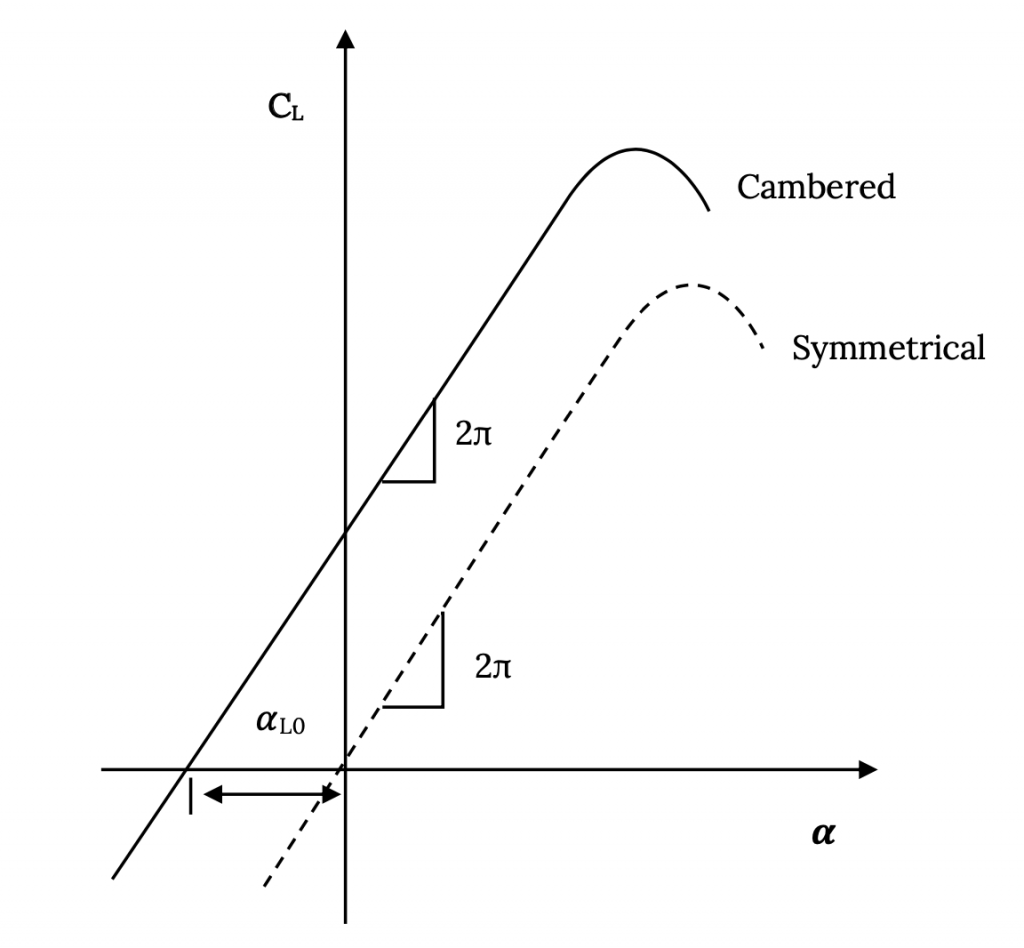
- The two dimensional lift coefficient will be CL = 2πα where α is the angle of attack (angle between the chord line and the free stream velocity vector).
For a cambered airfoil (non-symmetrical)
- The “center of lift” is not at the quarter chord and it, in fact, moves as angle of attack changes.
- The two dimensional lift coefficient will now be CL = 2π(α – αL0), where αL0 is called the “zero lift angle of attack” and is a negative angle for a positively cambered airfoil. This means that the lift curve shifts to the left as camber increases and that, at a given angle of attack, the cambered airfoil will produce a larger lift coefficient than the symmetrical airfoil (provided the airfoil is at an angle of attack below that for stall).
We talked about these same results in Chapter One without saying much about their origins. This shift in lift curve and increase in lift coefficient with increasing camber is the basis for the use of flaps as a temporary way to increase the lift coefficient when a boost in lifting capability is needed such as on landing.
The aerodynamic theory that would predict all this is called “thin airfoil theory” and it does this precisely as described above, by assuming that thousands of tiny vortices are laid side by side in what is called a vortex sheet along the airfoil’s camber line. Knowing the mathematical description of the shape of the desired camber line, the free stream velocity and the angle of attack, and requiring that there be no flow through the camber line and that the flow does not go from one surface to the other around the trailing edge, thin airfoil theory can tell the needed distribution of circulation along the camber line from leading edge to trailing edge to give a simulation of the real flow around the airfoil.
This method can’t predict stall. To do that we would need to consider the effects of shear or viscosity in the flow and this would require us to look at the “boundary layer” or viscous flow region around the actual wing surface. This too, is far beyond the scope of the material we want to investigate in this text.
So, is there a simple way to predict the effects of camber without resorting to thin airfoil theory of some equally messy procedure? It turns out that there is a “back of the envelope” method called “Weissinger’s Approximation”
3.2 Weissinger’s Approximation
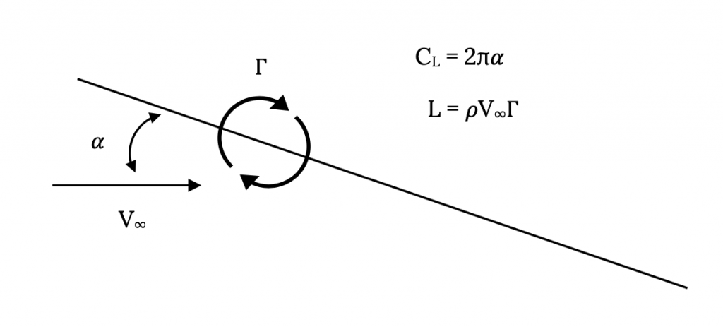
Weissenger’s Approximation is based on the symmetrical airfoil results of thin airfoil theory that were listed in a section above. These results say that for a symmetrical airfoil (essentially a flat plate) the lift acts at the quarter chord and the lift coefficient is 2-pi times the angle of attack.
We also have the Kutta-Joukowski Theorem which says that lift is equal to the flow density multiplied by the circulation and the freestream velocity.
We can, therefore, combine these two results by saying that we can model the lift on a flat plate by placing a single vortex at the quarter chord of the flat plate (since this is where theory says the net lift acts). All of this gives us the picture shown below.
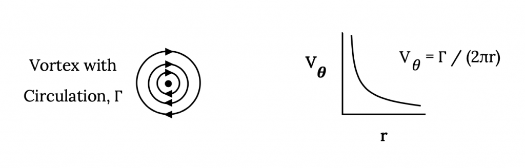
Basically, we are going to combine these two ideas that describe lift by selecting a place where we would impose a condition of no flow through the flat plate that will equate the lift from the two theoretical results. To do this we need to know something about a vortex that we have not previously introduced. That is, the velocity found in or introduced by a vortex at various distances from its center. Aerodynamic theory would tell us that the circular or tangential velocity in a vortex varies inversely with its radius and is a function of the circulation, Γ, in the vortex. Theoretically, a vortex has an infinite circumferential velocity at its center and this velocity gets smaller as we move further away from the center. This will give
Vvortex = Γ / (2πr)
In using this definition of the circumferential velocity in a vortex it is conventional in the field of aerodynamics to define the positive direction for Γ as clockwise. This defies conventional mathematical practice and care has to be taken in being consistent in using the convention.
This is illustrated below.
Going back to our combination of thin airfoil theory results and the Kutta-Joukowski Theorem we have the following task. We want to find some point on the flat plate where the vortex that we have placed at the quarter chord will give just the right amount of velocity to counteract the component of the freestream velocity normal to the plate such that our two looks at lift or lift coefficient will give the same answers. One theory, the Kutta-Joukowski Theorem tells us that L = ρV∞Γ and the other tells us that the lift coefficient CL = 2πα.
Realizing that the lift on a two dimensional flat plate is equal to the lift coefficient times the dynamic pressure, multiplied by the length of the plate (a “one dimensional area”), we can write:
L = ρV∞Γ = (2πα)(½ρV∞2)(c) ,
where “c” is the chord (length) of the flat plate.
It is easily seen that what is being sought here is a relationship between the angle of attack and the circulation in the vortex. We are relating the physical reality of lift increasing with angle of attack to the mathematical model that says lift increases with circulation.
Γ = παV∞c .
It is this relationship that we use to create our “back of the envelope model” called Weissinger’s Approximation. To see this we need to look again at our flat plate with the vortex at the quarter chord and ask ourselves at what radius from the vortex will the velocity from the vortex be just enough to balance the normal component of the freestream velocity.
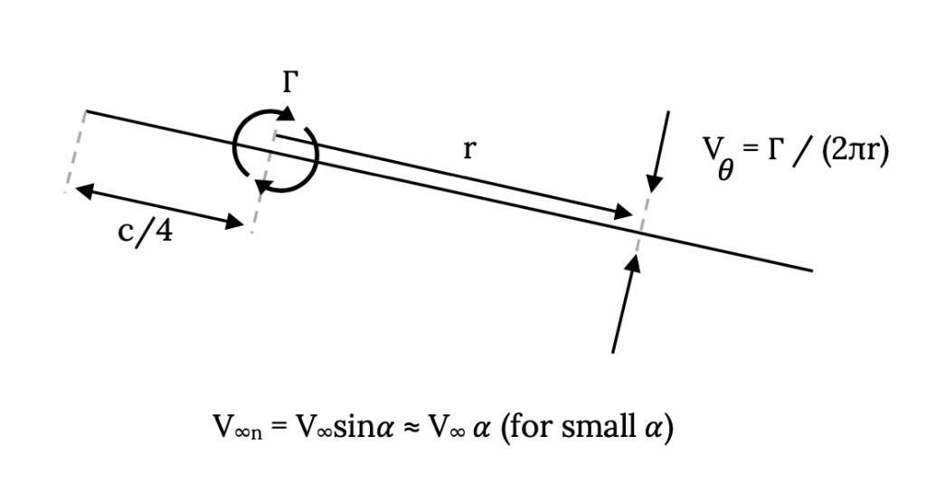
If we look at this illustration and use the last equation above to define the circulation, Γ, in terms of the freestream velocity and the angle of attack and then equate the velocity from the vortex and the normal component of the freestream velocity, we find
Vθ = Γ / (2πr) = (παV∞c) / (2πr) = V∞n = V∞ sin(α) ≈ V∞ α
or,
(αV∞c) / (2r) = V∞ α , for small angles of attack.
The final outcome of this is that the distance, r, at which we must solve for “no flow through the flat plate” to make the two theoretical models compatible is:
r = c/2 .
We must solve for no flow through the plate at a point three-fourths the way back (at the three-quarter chord point) to make this “approximation” work. We call this point the “control point”.
OK, so what’s the big deal? We’ve found a new way to get a result we already know and it is only for a flat plate! How can this “approximation” tell us anything we don’t already know?
The reason this is so useful is that we can “build” approximate models of cambered or flapped airfoils from flat plates. Consider the simple case of a symmetrical airfoil with a plain flap taking up the final 20% of its chord. We can model this as two sequential flat plates with one flat plate of length of 80% of the airfoil chord and the other 20% of the chord and we can deflect the “flap” and see what it does to the lift coefficient. The way this is done is illustrated in the figure below:
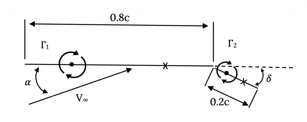
In the above case we will end up with two equations and two unknowns, the two values of circulation. To get these two equations we look at the flows normal to the two plates at their respective “control points” that have been placed at the ¾ chord points on each plate or panel. Lets look first at the control point on the first panel.
There will be three velocities that must be accounted for at this point; the component of the freestream velocity normal to the panel, the velocity induced by the vortex on the first panel, and the velocity induced by the vortex on the second panel. We can see in the figure below that the freestream velocity is directed upward while the velocities from the two vortices will be in opposite directions (that due to the first vortex is “down” and the velocity from the second vortex is “up”, if we assume the vortices are “positive” or clockwise). We can account for these directions by either mental bookkeeping and noting that they all must add to zero, or by conscientiously accounting for signs on the vector quantities, noting that the radii (r11 and r21) have signs related to their direction.
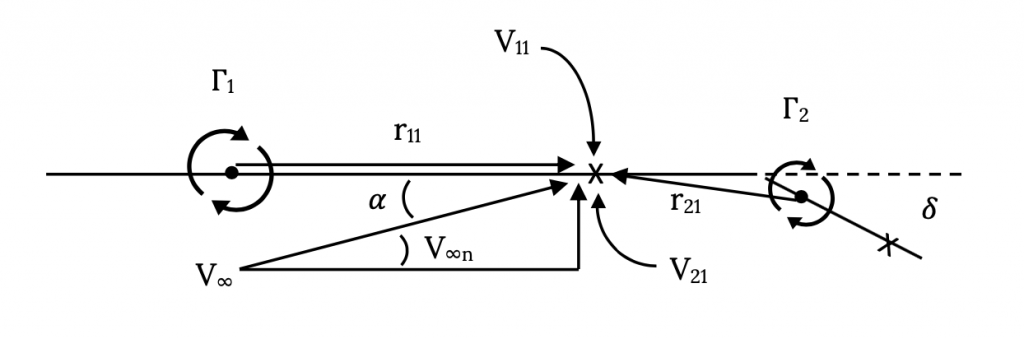
Note that the velocity induced at control point 1 by the vortex on panel 2 is not exactly perpendicular to panel 1. We could be very precise and use a little trigonometry to figure out the exact angle and account for it to find the true normal component or we could just assume it is close enough to normal to ignore the angle. Since this is an approximate method anyway, except in the case of very large angles (say ten degrees or more) we will usually ignore the error. Doing this, we can write an equation adding the two vortex components of velocity and equating their sum to the free stream component.
V11 + V21 = V∞n1 = V∞sin(α1) ≈ V∞ α1
where
V11 = Γ1 /(2πr11)
V21 = Γ /(2πr21)
and where
r11 = 0.4c
r21 ≈ – 0.25c
Now, we would do exactly the same thing at the control point on the second panel.
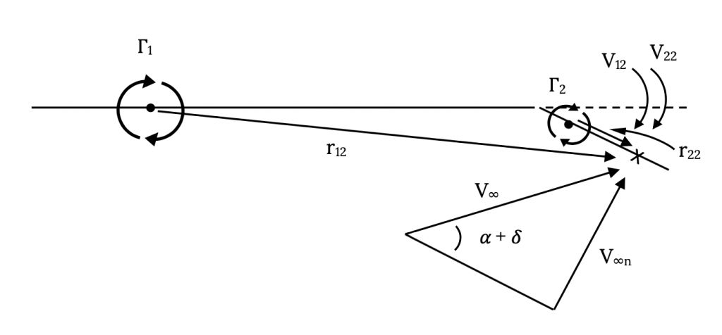
Here our equation will be similar to the one at the control point on panel one except that we will probably have to account for the fact that the flap deflection angle will probably be too large to simply ignore in finding the normal component of the freestream velocity.
V12 + V22 = V∞n2 = V∞sin(α2) = V∞sin(α + δ)
where
δ = flap deflection angle
V12 = Γ1 /(2πr12)
V22 = Γ2 /(2πr22)
r12 ≈ 0.75c
r22 = 0.1c
We would then simultaneously solve these two equations, each having two unknowns (Γ1 and Γ2) for those unknown values. We would then use those two values of circulation to find the total lift and lift coefficient where the lift would simply be found from the Kutta-Joukowski Theorem, summing the lifts on each panel.
L = ΣρV∞Γ = ρV∞ [Γ1 + Γ2]
and the lift coefficient would be
CL = L / (½ρV∞2c) = 2[Γ1 + Γ2] / (V∞c)
Exercise:
Solve the problem above for a freestream speed of 100 mph, a flap deflection of 20 degrees, and a 5 foot wing chord at sea level conditions at an angle of attack of 5 degrees. How does this lift coefficient compare with that for a symmetrical airfoil at the same angle of attack?
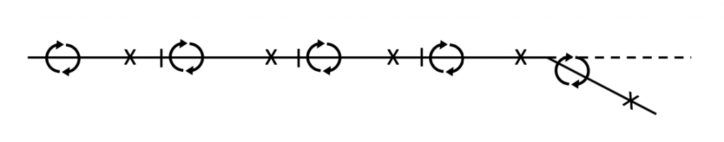
Note that in the above approximate solution for a flapped, symmetrical airfoil we have a very crude “lift distribution” over the airfoil chord, that is, we know the way lift can be divided to act at the two locations above. If we solved this for several different angles of attack we would find that the relative values of the two vortex strengths (circulations) would change. If we looked closely at this we would find that, unlike for the symmetrical airfoil where the lift can always be said to act at the airfoil quarter chord, for the cambered airfoil the point where the lift will act (center of lift or center of pressure) will move with angle of attack and will be a function of camber. If we wanted to find this more precisely we could use more panels and more vortices and control points (along with more equations). For the above example it might be natural to simply divide the airfoil into five panels of equal lengths, each 20% of the original chord, looking something like the sketch below.
And, it is not too hard to imagine extending this method to a truly cambered airfoil as shown in Figure 3.12.
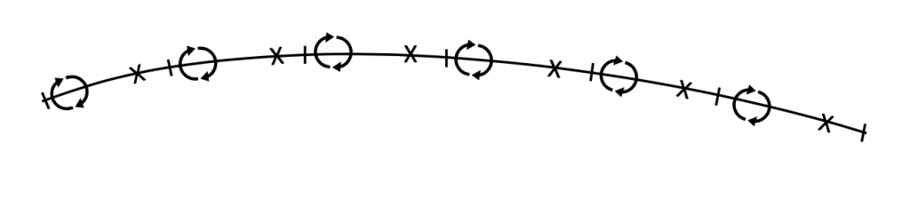
This simple approximation based on the results of flat plate aerodynamic behavior has, in this way, been stretched into a true “numerical solution” for an airfoil of any camber shape with as many panels as we wish to use. We can use it to find the total lift or lift coefficient for an airfoil with any camber shape and also to find the way lift is distributed over the airfoil chord.
Another thing we can find from this is the “pitching moment” of the airfoil, its tendency to rotate nose up or nose down about any desired reference point on the chord. The pitching moment is just found by taking each “lift” force found from the individual circulations and multiplying it by the distance or “moment arm” between that vortex and the desired reference point. If, for example, we want to use the leading edge of the wing as our moment reference (a common choice in theoretical or numerical calculations) we only need to take each value of gamma times the distance from the airfoil leading edge and that vortex and sum these to get the total pitching moment about the leading edge.
For the symmetrical airfoil (flat plate) where the center of lift is always at the quarter chord, this pitching moment around the leading edge will always be the lift multiplied by the quarter chord distance. The pitching moment coefficient for this case would be the lift multiplied by the quarter chord distance, divided by the dynamic pressure times the square of the chord. Do a quick calculation to see what this would be?
3.3 Pitching Moment
While we are talking about finding the pitching moment let’s take a look at some special cases. Pitching moment can be calculated or measured about any point we wish to use. Often in analytical or numerical calculations it is convenient to find the pitching moment around the wing leading edge. On the other hand, in wind tunnel testing it might be more convenient to measure the moment at some point between 20% and 50% back from the leading edge because of the ease of attaching the force and moment balance system there.
In Chapter One we mentioned two significant locations where the pitching moment or its coefficient has special meanings. These were the center of pressure (center of lift) and the aerodynamic center; points where the moment coefficient is zero or where it remains constant as the lift coefficient and angle of attack change. According to thin airfoil theory these are coincident at the quarter chord for a symmetrical airfoil but for the cambered airfoil, the center of pressure will usually move as angle of attack changes while the aerodynamic center remains at the quarter chord. We can verify that this theoretical result is a pretty good match for reality by looking at the aerodynamic data plots presented in Appendix A (discussed earlier in Chapter One). Often these plots present two graphs for pitching moment coefficient with the first one (on the left in most figures) a plot of CMc/4 (the moment coefficient at the quarter chord) and the other plot (usually on the right) of CMAC (moment coefficient at the aerodynamic center). In the plots in Appendix A for cambered airfoils it can be seen that CMc/4 is non-zero in value and changes with angle of attack while CMAC is relatively constant prior to the onset of stall. In the plots of symmetrical airfoil data both of these quantities are zero (or near zero) in value and constant prior to stall. In stall, the lift or pressure distribution over the airfoil is changing drastically as the flow begins to separate over progressively larger portions of the airfoil and the approximations of thin airfoil theory are far from valid.
As noted in the previous section, the pitching moment and moment coefficient can be calculated along with the lift when using the Weissinger Approximation. To find the location of the center of pressure we need only use the definition of that point as being where the moment is zero to find its location. Based on the illustration below, we can assume the center of pressure is located at some point Xcp and sum the moments about that unknown point due to the various circulation induced lift forces to equal zero.
ρV∞[Γ1(x1-xcp) + Γ2(x2-xcp) + • • • • + Γn(xn-xcp)] = 0
In this equation x1, x2, through xn are the locations along the chord of the various vortices (each at the quarter chord of its panel) and xcp is the unknown location of the center of pressure. This is solved for xcp, the location of the center of pressure. Note that for a symmetrical airfoil (flat plate) this position should not change with angle of attack while for a cambered airfoil xcp will be different for every angle of attack.
In a similar, but slightly more complicated fashion, we could find the location of the aerodynamic center from Weissinger Approximation lift results. This would involve finding the point where dCM/dCL = 0. We will leave this calculation for a text or course in aerodynamics.
3.4 Wings (3-D Aerodynamics)
As was pointed out in Chapter One, the main difference between two-dimensional flow around an airfoil and three-dimensional flow around a wing is the flow around the wing tip from the bottom to the top of the wing. This results in several things:
- An outward flow along the bottom of the wing near the tip.
- An inward flow along the top of the wing near the tip.
- A trailing vortex system.
- A “downwash” on the wing caused by the trailing vortex system.
- An “induced drag” caused by the downwash.
This vortex flow off of each wing tip is a very real flow that can be seen in the wind tunnel with either smoke or by simply sticking a string in the flow behind the wing tip. It can also be seen on airplanes in flight when atmospheric conditions are right. If there is sufficient moisture in the air in the form of high relative humidity or due to water vapor in the jet engine exhaust being pulled into the trailing vortices, the low pressure in the vortex core will cause the water vapor to condense, making it visible as a pair of “white tornados” trailing behind each wing tip. It is interesting to watch these when they are visible from high flying jets and to see just how long they persist. They can exist for many miles behind the generating aircraft, illustrating both the amount of energy in the vortices and the danger to other aircraft that might encounter them.
These “trailing vortices” are the key factor in trying to create any kind of mathematical model of the 3-D flow around and behind a real wing. In essence, this is done by bending the vortices that were used to model the flow over an airfoil at a 90 degree angle and allowing them to trail behind the wing. And, since we know that the lift on the wing varies along its span and doesn’t just stay the same all the way out to the wing tip, we allow vortices to turn right or left and come off the wing all along its span. This produces what is called a “horseshoe vortex system”.
While this theoretical derivation is beyond the intended scope of this material, its essence is found in the following facts or assumptions:
- The total circulation on the wing is assumed to vary along the span and to go to zero at the wing tips.
- The “trailing vortices” induce a downward flow or “downwash” that creates a small but significant downward velocity on the wing itself. (Actually, this is a way to account for the downward momentum of the flow that results from the lift force. This could also be found from the momentum equation if we had sufficient information.)
- In the same way that the interaction of the freestream velocity, V∞ , with the vortex circulations on the wing results in lift (Kutta-Joukowski Theorem), the interaction of this “downwash” velocity with the vortex circulations causes a drag. We call this the “induced drag”.
Using this horseshoe vortex model and assuming that all the vortices on the wing are bundled into a single, rope-like, core at the quarter chord of the wing and also assuming that the wing quarter chord is unswept, a method referred to as “lifting line theory” can be used to find the lift variation along the span and the induced drag for any unswept wing of moderate to high aspect ratio. Any good text on aerodynamics will have a full development of this approach to 3-D aerodynamics and will present its results.
One of the results of the use of lifting line theory will be an “optimum” case, that is, a spanwise lift distribution on the wing where the induced drag is a minimum. This turns out to be a solution where the spanwise distribution of circulation over the wing is elliptical in shape and mathematical form. This special solution will give the equation for induced drag coefficient that we have already cited in Chapter One,
CDi = CL2 / (πAR)
where “AR” is the aspect ratio,
AR = b2/S = b/cavg .
The more general (non-optimum) form of this equation for induced drag coefficient includes another term , “e” , known as Oswald’s efficiency factor, that accounts for non-elliptical spanwise variations of circulation.
CDi = CL2 / (πARe)
This Oswald’s efficiency factor can be calculated from lifting line theory in the form of a Fourier series.
While it is not the purpose of this text to go into much detail examining lifting line theory, I would like to briefly look at what it says about lift for the special, minimum drag, case of the elliptical lift distribution because we often use this special case to take a first look at the influences of wing design on aerodynamics and performance. Without deriving them, we will simply look at some of the most important results of lifting line theory related to lift:
L = (π/4)ρV∞bΓcenter
where
b = wing span
Γcenter = the value of the circulation at the center of the wing span
and
Γcenter = (2CLV∞S) / (πb)
Note that this makes the lift coefficient a function of the aspect ratio:
CL = L /(½ρV∞2S) = (πbΓcenter) / (2V∞S) = (π AR Γcenter) / (2bV∞)
This says that for any given angle of attack (or value of circulation since Γcenter must increase with angle of attack) a higher aspect ratio wing design will give a higher lift coefficient than a low AR wing.
If we plot lift coefficient versus angle of attack for two wings of different aspect ratio we would find that the “slope” of the lift curve would decrease with decreasing aspect ratio. The maximum value of the slope is 2-pi, the two dimensional airfoil value, equivalent to an infinite aspect ratio wing.
Another way to look at this same effect is to look at the angle of attack at which two wings of different aspect ratios must be flown to get the same value of lift coefficient:
α2 = α1 + (CL/π) [(1/AR2) – (1/AR1)]
The above relationships give us valuable tools for examining the effects of design variables like wing aspect ratio on the aerodynamics and performance of an aircraft. Should we wish to use a moderate aspect ratio wing instead of a high aspect ratio design for, say, structural reasons or for improved roll dynamics, we can see what penalty we will pay. Often the penalty may not be as great as we might at first believe based on our basic knowledge that high aspect ratio is usually desirable.
These equations are, as mentioned earlier, for the ideal case, the elliptical lift distribution or minimum induced drag case. Nonetheless, they can give us a pretty good idea of how things like changes in aspect ratio will influence the performance of any three-dimensional wing.
One final thing I would like to mention in this chapter relates to the assumptions mentioned earlier for lifting line theory. It was noted that this theory assumes that the quarter chord of the wing is unswept. Another assumption inherent in the use lifting line theory that was not mentioned is that the theory is not very good for low aspect ratio wings. Even with these two important limitations, lifting line theory gives us some important insights into 3-D aerodynamics. But, what would we do if we are looking at a wing with sweep or low aspect ratio?
For swept wings, wings with low aspect ratio, or any other wing beyond the bounds of the assumptions of lifting line theory, the usual approach is to go to some variation of what is called “vortex lattice” theory. The wing (or even the entire airplane) is divided into panels and a single “horseshoe” vortex is placed at the quarter chord of each panel in what is essentially a three-dimensional version of Weissinger’s Approximation. If the wing is broken into N panels, there are N horseshoe vortices and these must be solved by setting up N equations. The equations are solved for the condition of no flow through the panels (the same idea as with Weissinger’s Approximation) at the center span of the three-quarter chord of the panel. This solution is three times as complex as the 2-D Weissinger method because each horseshoe vortex has three segments (one spanning the panel’s quarter chord and the other two acting as “trailing vortices” from the first vortex at the panel’s edges. Just as in the 2-D method, the equations solved at the “control points” had to account for all the velocities induced by all the vortices on the airfoil as well as the freestream velocity, in the 3-D vortex lattice approach the equation at each panel’s control point must account for the velocities induced by all three vortex segments from all N panels as well as for the freestream velocity.
Vortex lattice methods can be intimidating at first; however, like the Weissinger Approximation in 2-D, they merely use N equations to solve for N unknowns where the unknown is the strength of the horseshoe vortex on each 3-D panel. Everything else boils down to modeling the geometry of the 3-D wing. The result will be the 3-D velocity vector parallel to each panel control point and these can be used to find the pressures and forces and moments all around the wing.
3.5 Vortex Aerodynamics: Winglets
We will look at one final subject in this chapter, that of “vortex aerodynamics”. As we have already seen, vortices play a major role in the way we mathematically model airfoil and wing aerodynamics. And, as we have seen in the case of three dimensional flows around wing tips, vortices actually play a very real role in creating things like lift and drag and the math models we construct to explain aerodynamics also do an excellent job of modeling these real vortices and their effects.
There are many situations in addition to the wing tip vortices where these tornado-like flows exist in “real life” and play a major role in creating forces and moments on airplanes and wings. One of the jobs of the aerodynamicist is to correctly model these vortices and their effects and another job may be to determine if there are ways to use these swirling flows to our advantage in ways that will improve an airplane’s aerodynamics and flight performance.
We will look at two very important and interesting cases where vortex aerodynamics plays important roles. These are in the use of “winglets” and “leading edge extensions” (sometimes known as “strakes” or “wing gloves”).
The winglet is, by now, a fairly well known addition to the wing tips of many airplanes but its purpose is widely misunderstood. For many, many years engineers and scientists tried many approaches that might reduce the strength or effects of wing tip vortices or that would eliminate them altogether. Unfortunately, the laws of Physics are hard to overcome, and this rotational energy that we quantify as “circulation” has to go somewhere at the wingtip and there is really no way to eliminate it in flight other than to let it slowly dissipate as a trailing vortex pair somewhere in the atmosphere far downstream of the aircraft. We can put big plates on the wingtip or create interesting wingtip shapes iin attempts to eliminate or hasten the dissipation of the trailing vortices but the usual effect is simply to create a slightly different circular of tangential velocity distribution within the vortex itself, a pattern that may or may not make the vortices less dangerous to trailing aircraft and may or may not result in any reduction in the wing’s induced drag. Usually the effects of such “fixes” are greater in their inventor’s imagination than in real life.
The winglet, more properly known as the Whitcomb winglet after their inventor, Richard Whitcomb of NASA-Langley, is, contrary to conventional wisdom, not designed to eliminate the wingtip vortices. Rather than try to eliminate something that can’t be eliminated without eliminating the wing’s lift, Whitcomb decided to use the trailing vortices to create a positive effect. In a conversation with the author, Mr. Whitcomb explained that he saw the winglets as working much like the keel on a sailboat that is sailing or “tacking” into the wind. A sailboat keel is a kind of wing on the bottom of the boat, and when a sailboat is sailing into the wind, the forward force is not coming from the sail at all. Instead, the sail is creating a sideward force that pushes the keel through the water in such a way as to create a forward directed force. The forward force pushing a sailboat into the wind is coming from a small wing in the water rather than from the large wing we call a sail.
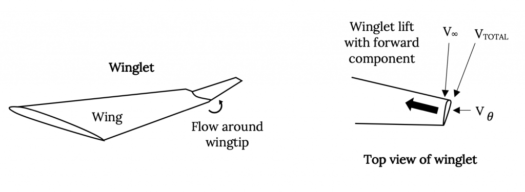
In creating the winglet, Richard Whitcomb reasoned that if the large wing on a sailboat could create a flow over a smaller wing (the keel) that would produce a thrust, there ought to be a way to take the flow created by a large wing on an airplane (the tip vortex) and use it to create a thrust on a smaller wing. That smaller wing ended up being the winglet. The Whitcomb winglet is placed at what would appear to be a negative angle of attack on the wingtip such that the combination of the freestream velocity and the wingtip vortex flow velocities creates a “lift” on the winglet that is actually pointed forward, giving a thrust. And it turns out that this thrust is significant enough to improve the lift-to-drag ratios on a wing by fifteen to twenty percent. This can result in very significant improvements in airplane flight performance and economics.
3.6 Vortex Aerodynamics: Leading Edge Vortex
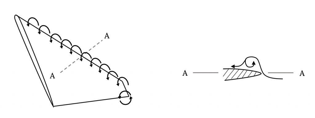
The second type of real vortex that we want to examine very briefly is the “leading edge vortex”. Such a vortex forms when a wing is swept to angles of about 50 degrees or more. These vortices, illustrated in figure 3.18 below, result from a combination of a three-dimensional, spanwise flow on the wing and from the normal flow around the leading edge of the wing. This combined flow actually separates from the wing surface at the leading edge but, due to the rotational flow in the vortex, reattaches to the wing surface in such a way that the wing does not stall at the usual fifteen to twenty degree angle of attack but has attached flow and lift up to much larger angles of attack.
Wings are usually swept to delay the onset of the transonic drag rise near Mach One and to reduce the magnitude of that drag rise. On the other hand, swept wings produce less conventional lift at a given angle of attack than an unswept wing, in much the same manner as lower aspect ratio wings give less lift at a given angle of attack than high aspect ratio wings. The effect of the leading edge vortex is two-fold. First, by keeping the flow attached to much higher than normal angles of attack, they enable the wing to produce lift at these higher than normal angles of attack. Added to this increased angle of attack advantage is an extra lift, called “vortex lift” that is created by the very low pressure at the vortex core. Unfortunately, this low pressure in the vortex also adds some drag, but the net effect can be very useful in allowing airplanes that need highly swept wings to operate efficiently at transonic and supersonic speeds to still get the lift they need at lower subsonic speeds. They also can allow military fighter airplanes to “fly” at very unusual attitudes (angles of attack) that can be very useful in air-to-air combat.
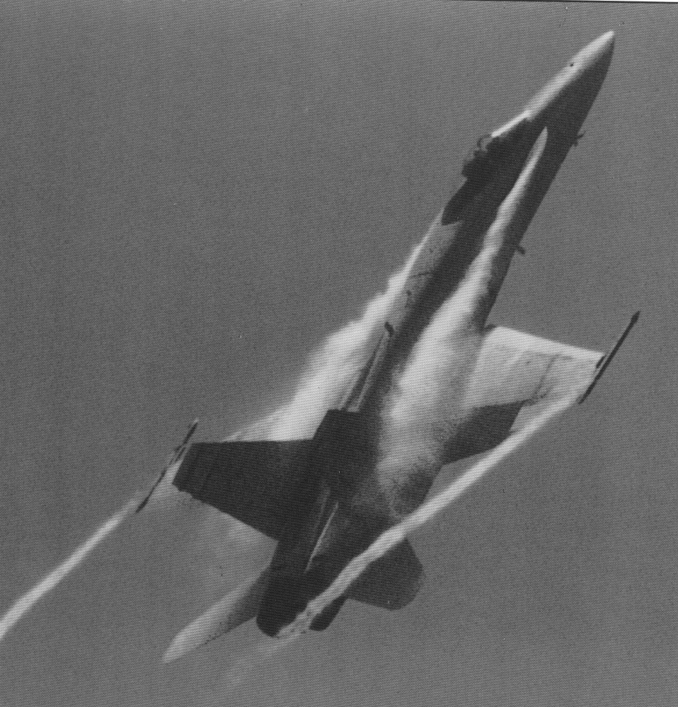
Sometimes we want to create this same capability on wings that aren’t swept that much. This can be done by adding highly swept leading edge extensions or strakes. These strakes create their own leading edge vortices which continue over the wing behind them, giving many of the benefits mentioned above and allowing airplanes with relatively low wing sweep to fly at much higher than normal angles of attack when needed. One airplane that makes good use of this effect is the Navy’s F-18. Its very long and highly swept strakes enable it to operate at the high angles or attack and low speeds needed for landing and takeoff on aircraft carriers while also giving it very useful high angle of attack maneuverability that is very useful in fighter combat.
As was mentioned at the beginning of this chapter, the coverage in the chapter is not really needed to be able to understand or work with the material on aircraft performance that will follow. It has been included simply to fill in some of the blanks that might have been left open in Chapter One. On the other hand, it can be used to enhance the following aircraft performance coverage and to better relate it to some of the basic concepts in aerodynamics.
Homework 3
1. The Airbus 380-100 is designed to cruise at 35,000 ft at a Mach number of 0.85. Its weight in cruise is approximately one million pounds. It has a wing area of 9100 ft2 and a wing span of 262 ft. Assuming that lift equals weight and thrust equals drag and that in cruise at this altitude 50,000 pounds of thrust is needed, find:
a. The flight speed in miles per hour and in knots
b. The lift coefficient
c. The drag coefficient
d. Its Reynolds number based on mean chord
2. If an airplane is taking off by simply accelerating down the runway until it has sufficient speed for its lift to equal its weight and its wing is at a five-degree angle of attack, what speeds are required for takeoff at sea level and at 5000 feel altitude assuming that its wing has a lift curve slope (dCL/dα) of 0.08 per degree and a zero-lift angle of attack (αL0) of minus one degree? Also find the indicated airspeed at both altitudes. Assume the airplane weighs 11,250 pounds and has a wing area of 150 ft2.
Note: Normally most aircraft would accelerate at a low value of lift coefficient and then “rotate” to increase their angle of attack to a value that will give lift + weight at the defined take-off speed. This would allow take-off in a shorter distance than the method above. We will look at this in detail later in the course.
References
Figure 3.1: Kindred Grey (2021). “Upper and Lower Surface Speed Difference Gives Lift.” CC BY 4.0. Adapted from James F. Marchman (2004). CC BY 4.0. Available from https://archive.org/details/3.1_20210804
Figure 3.2: Kindred Grey (2021). “Model of Upper and Lower Surface Speed Difference.” CC BY 4.0. Adapted from James F. Marchman (2004). CC BY 4.0. Available from https://archive.org/details/3.2_20210804
Figure 3.3: Kindred Grey (2021). “Modeling Airfoil Flow With Multiple Vortices .” CC BY 4.0. Adapted from James F. Marchman (2004). CC BY 4.0. Available from https://archive.org/details/3.3_20210804
Figure 3.4: Kindred Grey (2021). “Lift Coefficient Curves for Symmetrical and Cambered, 2-D Airfoils.” CC BY 4.0. Adapted from James F. Marchman (2004). CC BY 4.0. Available from https://archive.org/details/3.4_20210804
Figure 3.5: Kindred Grey (2021). “Basic Sketch and Equations for Weissinger’s Approximation.” CC BY 4.0. Adapted from James F. Marchman (2004). CC BY 4.0. Available from https://archive.org/details/3.5_20210804
Figure 3.6: Kindred Grey (2021). “Mathematical Model of a Vortex.” CC BY 4.0. Adapted from James F. Marchman (2004). CC BY 4.0. Available from https://archive.org/details/3.6_20210804
Figure 3.7: Kindred Grey (2021). “Solution Method fo Weissinger’s Approximation.” CC BY 4.0. Adapted from James F. Marchman (2004). CC BY 4.0. Available from https://archive.org/details/3.7_20210804
Figure 3.8: Kindred Grey (2021). “Use of Two Panel Weissinger Method for Flapped Airfoil.” CC BY 4.0. Adapted from James F. Marchman (2004). CC BY 4.0. Available from https://archive.org/details/3.8_20210804
Figure 3.9: Kindred Grey (2021). “Solution Method at the First Control Point.” CC BY 4.0. Adapted from James F. Marchman (2004). CC BY 4.0. Available from https://archive.org/details/3.9_20210804
Figure 3.10: Kindred Grey (2021). “Solution Method at Second Control Point.” CC BY 4.0. Adapted from James F. Marchman (2004). CC BY 4.0. Available from https://archive.org/details/3.10_20210804
Figure 3.11: Kindred Grey (2021). “Five Panel Weissinger Sketch for Flapped, Symmetrical Airfoil.” CC BY 4.0. Adapted from James F. Marchman (2004). CC BY 4.0. Available from https://archive.org/details/3.11_20210804
Figure 3.12: Kindred Grey (2021). “Weissinger Method for Cambered Airfoil.” CC BY 4.0. Adapted from James F. Marchman (2004). CC BY 4.0. Available from https://archive.org/details/3.12_20210804
Figure 3.13: Kindred Grey (2021). “Finding the Center of Pressure.” CC BY 4.0. Adapted from James F. Marchman (2004). CC BY 4.0. Available from https://archive.org/details/3.13_20210804
Figure 3.14: Kindred Grey (2021). “Horseshoe Vortex System.” CC BY 4.0. Adapted from James F. Marchman (2004). CC BY 4.0. Available from https://archive.org/details/3.14_20210804
Figure 3.15: Kindred Grey (2021). “3-D Aspect Ratio Effects on Lift Curve Slope.” CC BY 4.0. Adapted from James F. Marchman (2004). CC BY 4.0. Available from https://archive.org/details/3.15_20210804
Figure 3.16: James F. Marchman (2004). “Sketch of Vortex Lattice Paneling Method.” CC BY 4.0.
Figure 3.17: Kindred Grey (2021). “Winglet Operation (a) Winglet.” CC BY 4.0. Adapted from James F. Marchman (2004). CC BY 4.0. Available from https://archive.org/details/3.17_20210804
Figure 3.18: Kindred Grey (2021). “Leading Edge Vortex.” CC BY 4.0. Adapted from James F. Marchman (2004). CC BY 4.0. Available from https://archive.org/details/3.18_20210804
Figure 3.19: James F. Marchman (2004). “Vortex Flows on an F-18 (NASA Photo).” CC BY 4.0.
