Chapter 24. Using Surface Constraints

The prior chapter covered creating surface constraints in a LAS dataset. This chapter covers surface constraints in analysis by demonstrating the use of surface constraints to create digital elevation models (DEMs). This chapter does not discuss which method and surface constraint is best to use when creating a DEM. For that discussion, please consult the appropriate academic literature and/or project instructions.

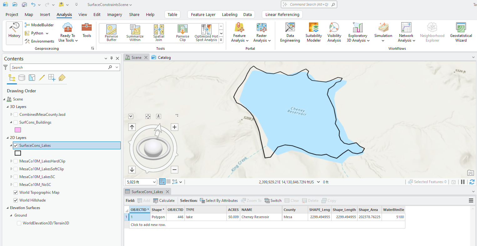
Create a new local scene project and add the Combined Mesa County .lasd file that has all six tiles. Add the lakes surface constraints feature class created in Chapter 23. Creating Surface Constraints. The building feature class can also be added for reference purposes only.

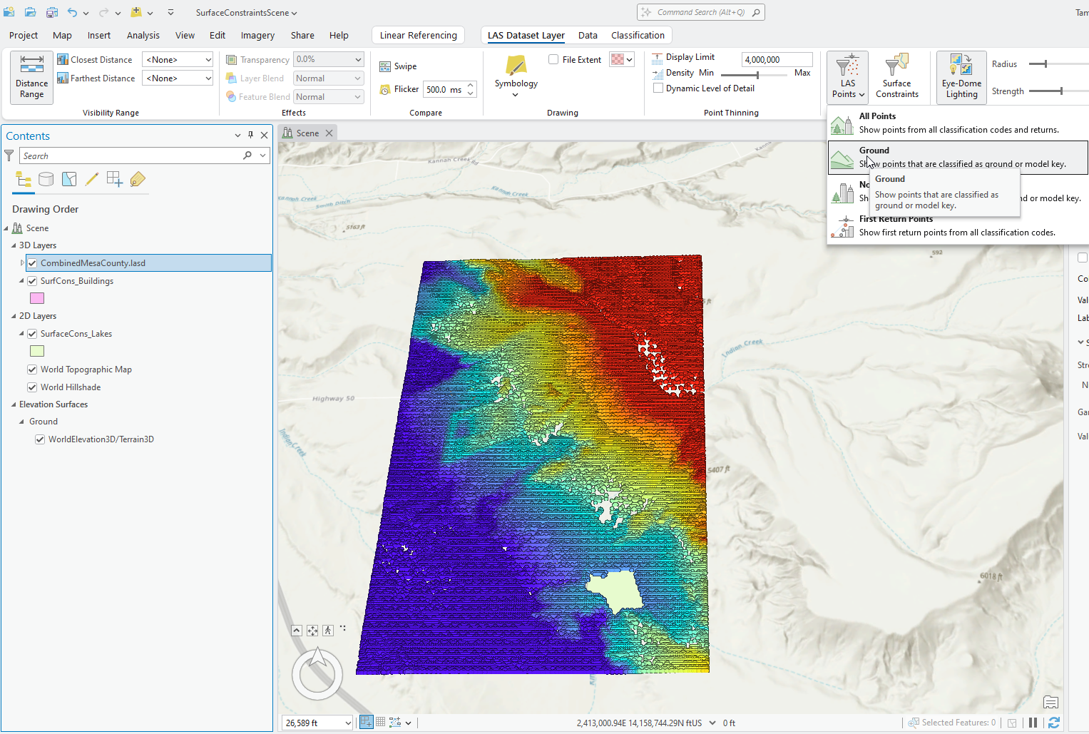
If both feature classes are added, notice that the Lakes feature class is listed under 2D layers and Buildings under 3D. Why? Remember, Buildings has an elevation field in its attribute table, so it can be displayed in 3D.  Select the LAS dataset and under Las Dataset Layer > Appearance > Las Points, choose Ground (Figure 24.1).

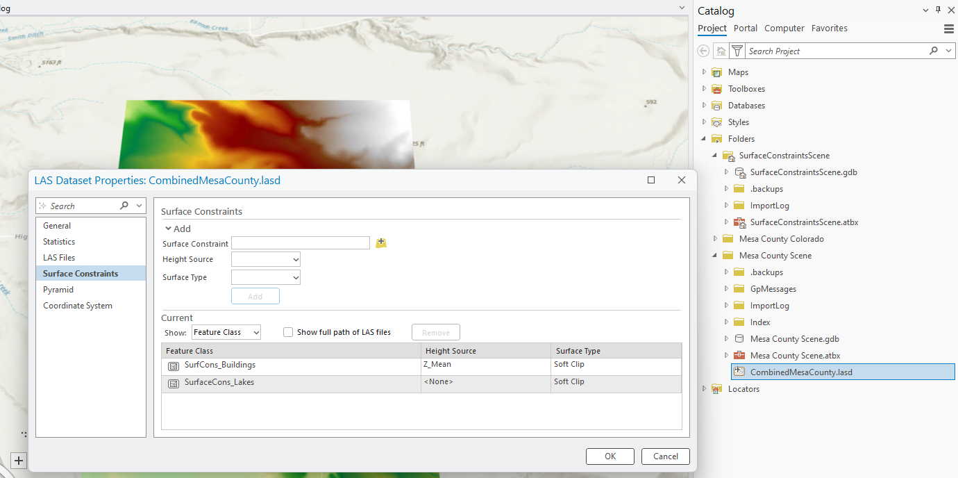
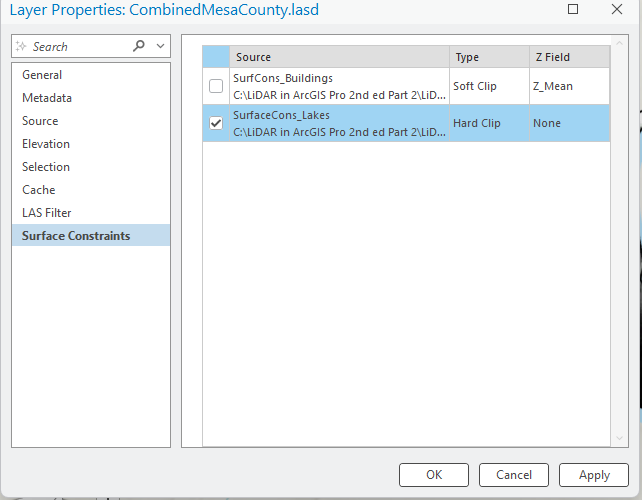
Ensure no surface constraints are checked under Properties > Surface Constraints (Figure 24.2). If none are showing, that is fine, the surface constraints will be changed as this chapter proceeds.

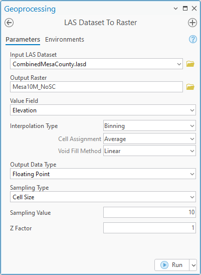
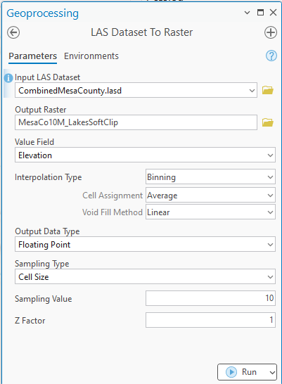
Create a 10-meter digital elevation model with no surface constraints using the LAS Dataset to Raster tool. Leave the defaults for all settings (Figure 24.3).

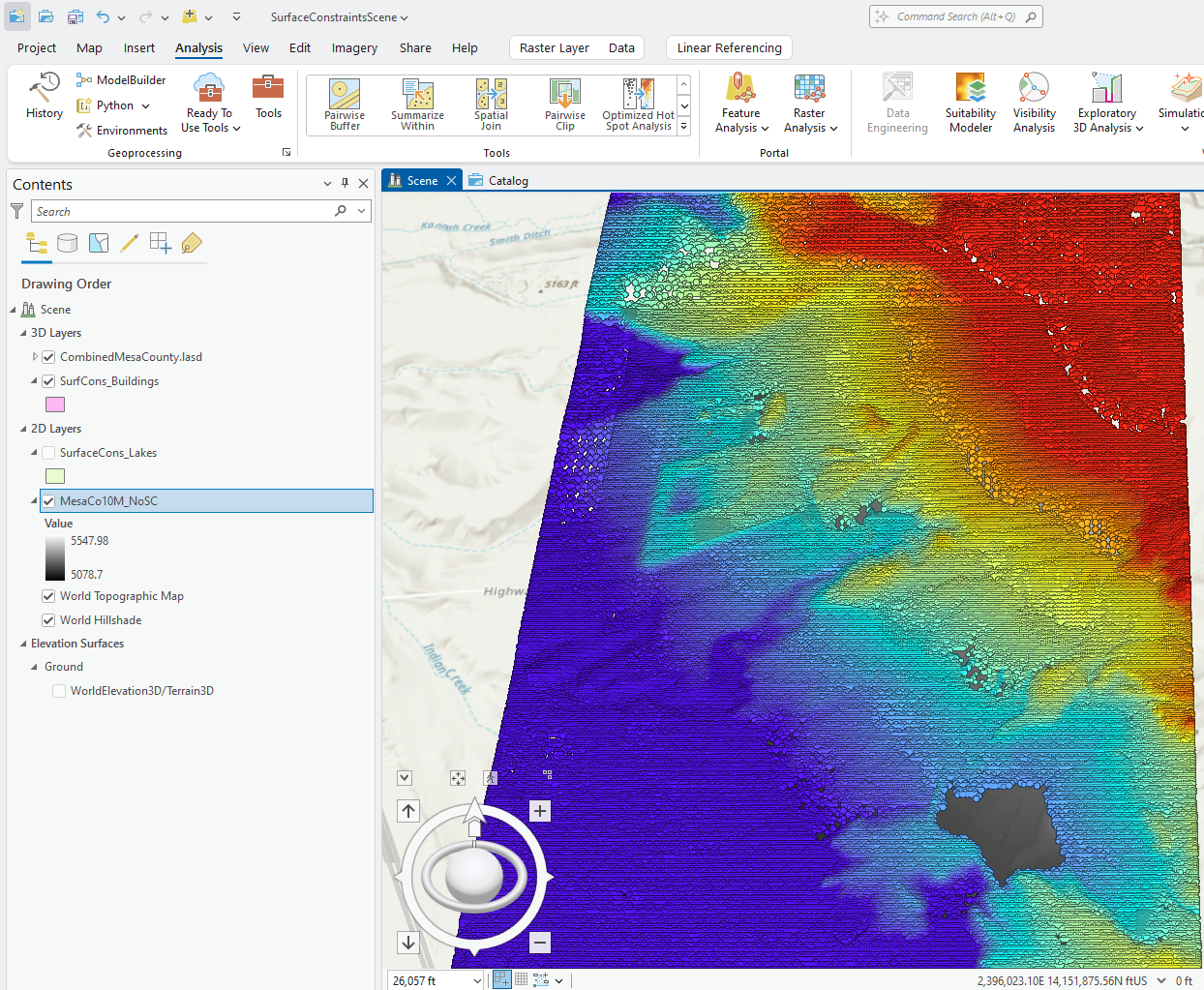
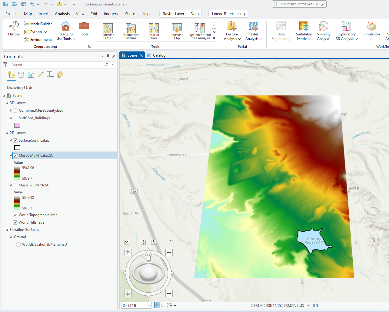
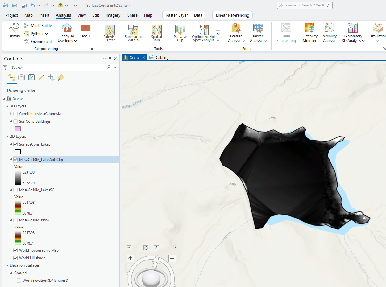
The results are added under 2D Layers in Contents (Figure 24.4).

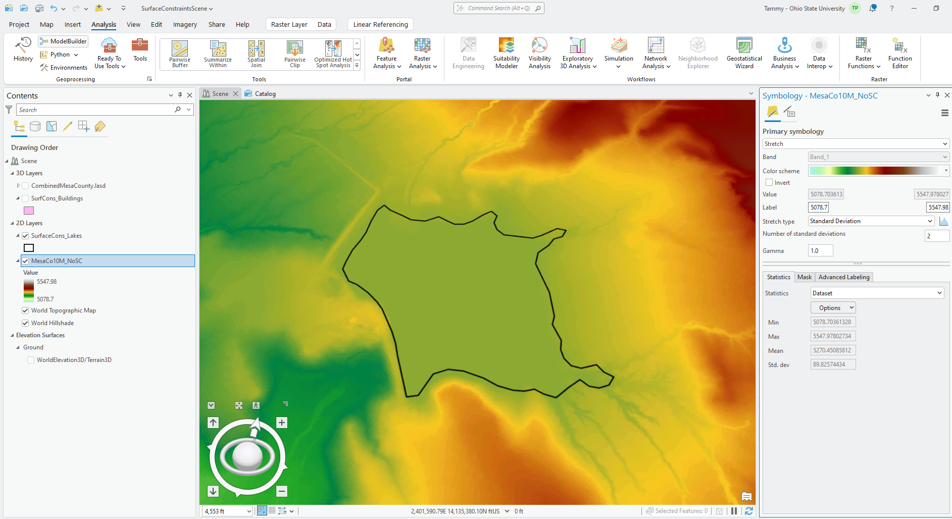
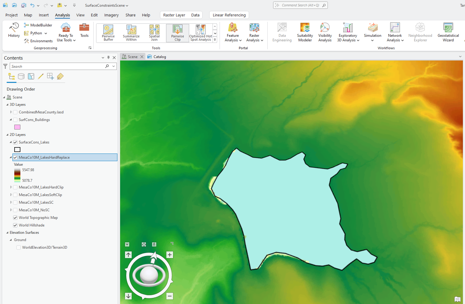
Turn off the 3D Layers (including the .lasd file), zoom to the lake, and change the symbology to Elevation #1  for the Color Scheme and Standard Deviation for the Stretch Type, so the lake is visible. The lake and feeder streams are visible in the map. Figure 24.5

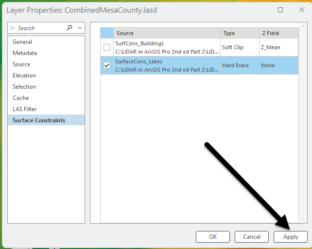
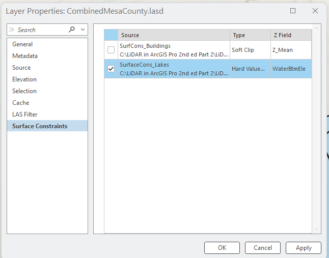
If Lakes is not already added as a Surface Constraint with a Hard Erase, add it (See Chapter 23 if you don’t remember how to do this). In the Combined Mesa County LAS Dataset, open the Properties>Surface Constraints tab and place a check mark in the box by the Surface Constraints Lake Feature Class (Figure 24.6).  Click Apply.

Now run the LAS Dataset to Raster tool again, leaving the default settings for now (Figure 24.7). This demonstration illustrates what happens when there is no elevation value in the feature class and a hard erase is used. Once the tool is filled as shown, Run the tool.

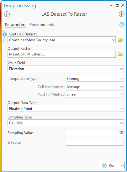
Figure 24.8 shows the result. The image initially displays in gray scale. Change the symbology to Elevation #1.

What happened? Using a hard erase left a hole where the lake is located—the tool was instructed to erase any values within the lakes polygon. You may need to turn off the first DEM to see the change.

Would a Soft Erase make any difference? Change the Surface Constraint to Soft Erase and run the tool again with the same default values. There is not a noticeable difference in the result (Figure 24.9). Again, the tool was told to erase (eliminate) those values, so it left a hole in the DEM.

Change the Surface Type to Soft Clip. Remember from Chapter 23, go to Catalog, remove the prior Surface Constraint and add a new one with the Soft Clip type (Figure 24.10).

Go back to Scene view. Go to Properties > Surface Constraints to place the check mark to apply the constraint! Then run the tool again. Be sure to name the file appropriately. Use all of the defaults in the tool (Figure 24.11).

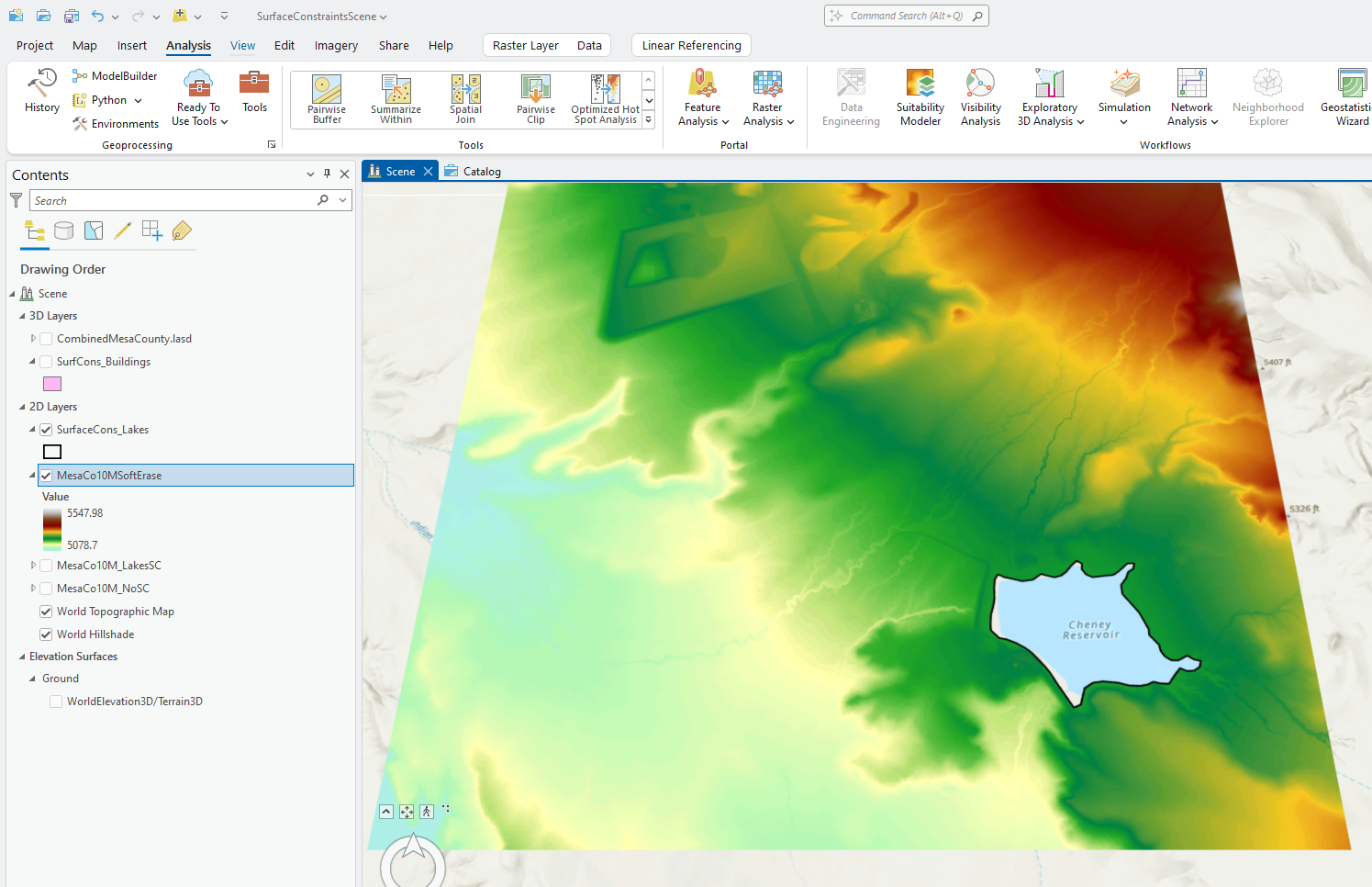
The results are shown in Figure 24.14. Remember, this is a clip, so it clipped the DEM to the extent of the Lakes feature class.

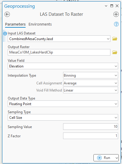
Redo the clip with a Hard Clip and the same parameters in the tool (Figure 24.13). Remember you first need to change the surface constraint type (Figure 24.14).

What is the difference between an Erase and a Clip? An Erase removes all the data within the polygon, it leaves a hole in the resulting new data where the polygon (the lake in this example) is located. A Clip removes all the data outside of the polygon, so the shape that is left is that of the lake itself.

What is the difference between Hard and Soft? There is no difference in the appearance of the resulting DEM, or other raster generated from the LAS dataset with surface constraints. The difference occurs when the new raster is used in another operation such as creating a TIN (triangular irregular network) ^[1]. For a further discussion on this, reference the ArcGIS Pro® online support at https://pro.arcgis.com/en/pro-app/latest/help/data/tin/tin-in-arcgis-pro.htm

What happens if there is an elevation field in the surface constraint feature?

Let’s examine.  First, add a field to the attribute table, called Water Bottom Elevation (abbreviate it WaterBtmEle) and calculate the field at 5100 (ft). The building file has multiple elevation fields, but practice is always recommended when learning any GIS tool. (Figure 24.15)

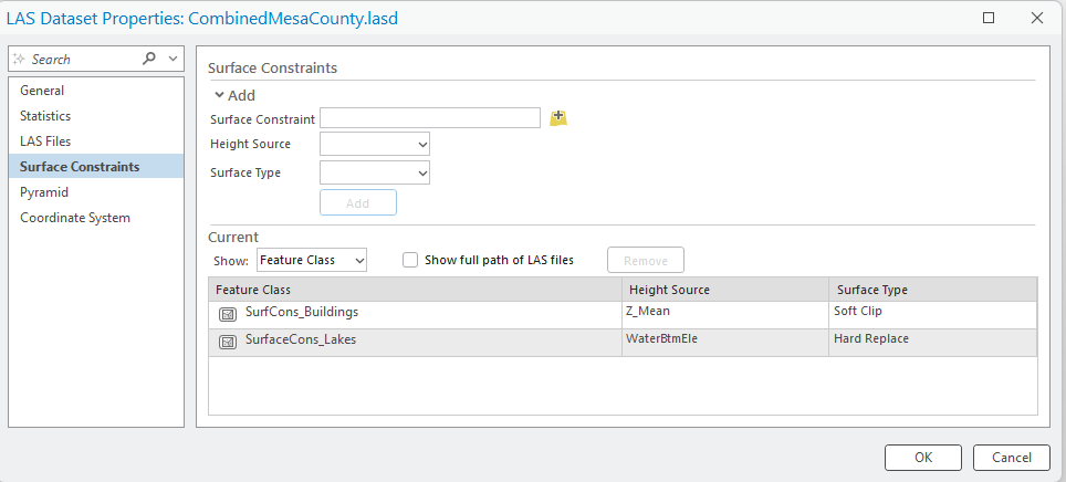
Remove the old surface constraint and add a new one with the Height Source as WaterBtmEle and the Surface Type as Hard Replace (Figure 24.16). Remember that most of the lake is missing lidar points. A lake’s bottom is not necessarily level but remember this is a reservoir, a manmade lake meant to hold water. It was excavated, and likely the original bottom depth was uniform when built. And since it is just one polygon, only one depth value (or bottom elevation value) can be used.

Don’t forget to check the box in front of the constraint in Properties > Surface Constraints and Run the LAS Dataset to Raster tool using the default values (Figure 24.17).

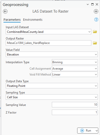
Figure 24.18 displays the result (Symbology changed to Elevation #1 and Standard Deviation as in the first DEM generated in this chapter). The lake is all one color because all the raster values for the lake are the same.

This chapter will not demonstrate Soft Replace, but feel free to run the tool. The result will be the same.

Let’s do one final demonstration—Hard Value Fill (Figure 24.19).

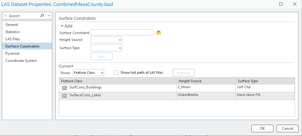
Again, be sure to check the constraint within the Properties>LAS Constraints tab (Figure 24.20).

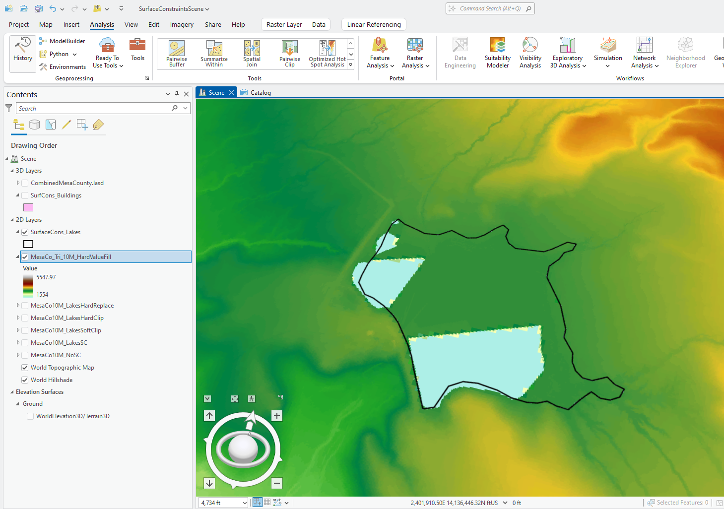
Instead of the default values, use Triangulation (the default method, Binning, should return the same result as the prior two DEMs). When changing the Interpolation Type to Triangulation, the Interpolation Method automatically changes to Linear and Thinning Type to No Thinning. Do you remember what Thinning is? It thins out the lidar points in the point cloud. When creating a DEM use No Thinning unless the project specifically requires it. Once the LAS Dataset to Raster tool is filled as shown in Figure 24.21, select Run. This tool takes a bit longer to run than when running the tool with the defaults.

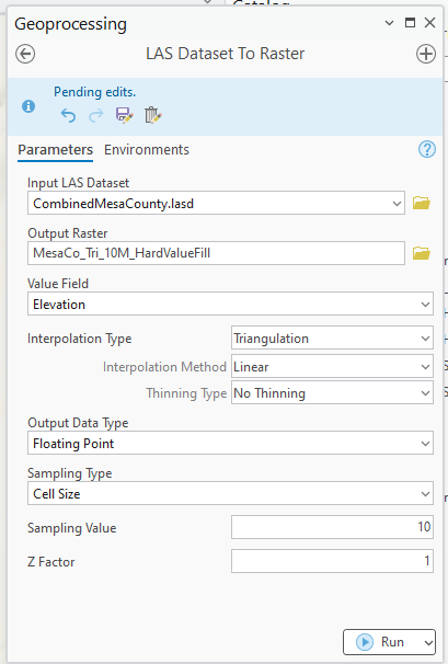
Figure 24.22 shows the result. The DEM outside of the Lake is unchanged. The method used to fill in the lake values, linear interpolation, used point values both from surrounding the lake and within the lake.

This chapter was strictly demonstrating the step-by-step process for using surface constraints. It does not demonstrate any additional surface constraint types or any other type of GIS analyses that can be generated with surface constraints and a LAS dataset.

When should surface constraints be used? Again, it depends on the parameters of the project or in the case of new research—the academic literature.