Prior chapters omitted surface constraints. Surface constraints are created using vector feature classes that represent a feature in the area covered by the lidar point cloud, such as trees, water bodies, buildings, etc. Surface constraints can be points, lines, or polygons (shapefiles or feature classes). One LAS dataset can reference multiple vector files for surface constraints. Surface constraints can be included when creating a LAS dataset or can be added later. Surface constraints place processing or classification limitations, which can vary in type. These limitations will be discussed in this chapter.

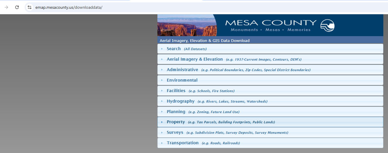
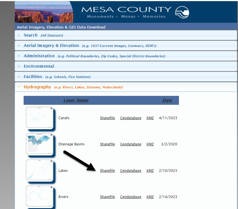
First, some vector files are needed for surface constraints. Go to the Mesa County Colorado GIS Download site at https://emap.mesacounty.us/DownloadData/ (Figures 23.1 and 23.2).

Under Hydrography, download the Lakes Shapefile (Figure 23.2).

Under Property, download the BLM Properties and Building Footprints Shapefiles (Figure 23.3).

Once all three shapefiles are downloaded, unzip them and save them.

Create a new map (not a scene) and add the Mesa County LAS dataset created in Chapter 14. Adding Tiles to an Existing .lasd Dataset.

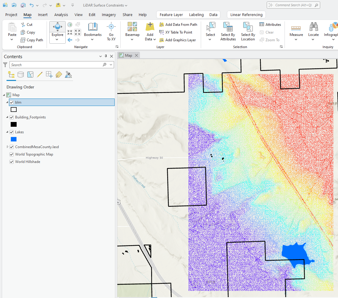
Add the three shapefiles—Buildings, BLM and Lakes (Figure 23.4). Ensure the LAS dataset is added first so the map is zoomed in to the lidar data extent and not Mesa County. Change the symbology on the three vector layers so the footprints are distinct. One lake and five buildings are displayed within the footprints of the lidar tiles. The Lakes and Building_Footprints layers will be used to create surface constraints. The BLM layer is strictly reference information.

Since the study area is not all of Mesa County, all of the buildings and lakes in Mesa County are not needed. Using interactive selection, we will select only the buildings and lakes within the footprint of the lidar point cloud.

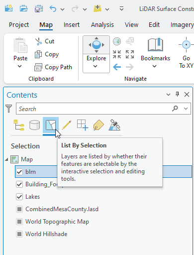
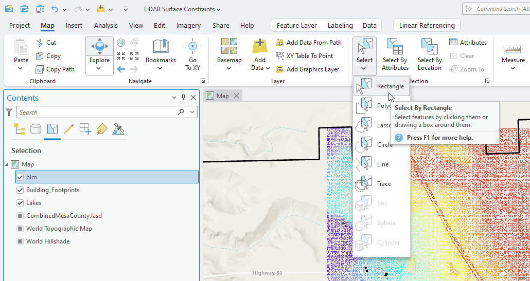
First, change the Contents view to List by Selection (Figure 23.5).

Under the Map tab on the ribbon, click the down arrow under Select, and choose Rectangle (Figure 23.6).

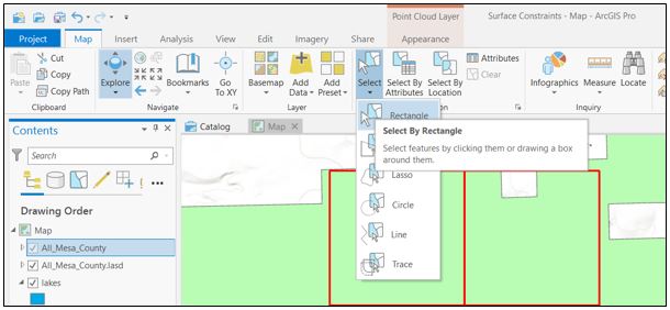
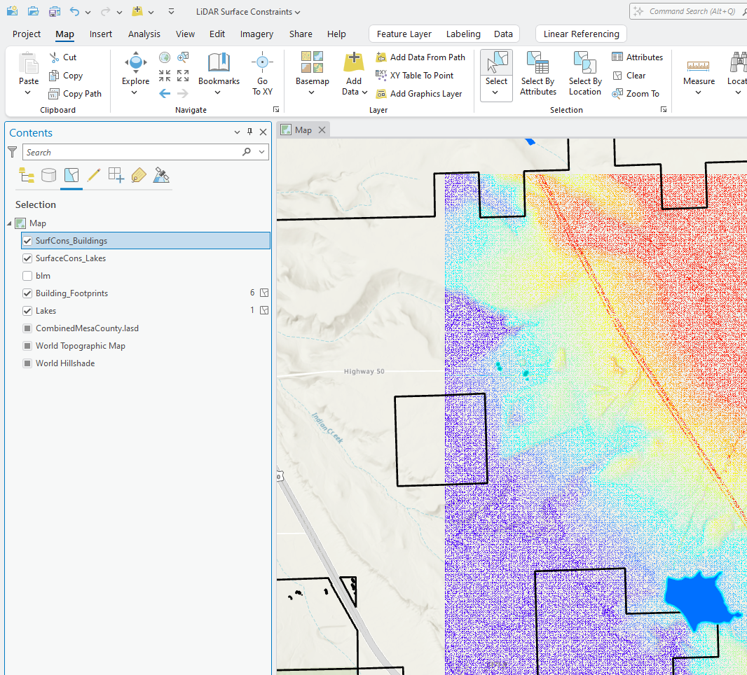
In the map viewer, drag from the upper left corner of all six lidar tiles to the lower right corner of the tiles. One lake and five buildings should be highlighted in cyan and show as selected features in Contents (Figure 23.6).

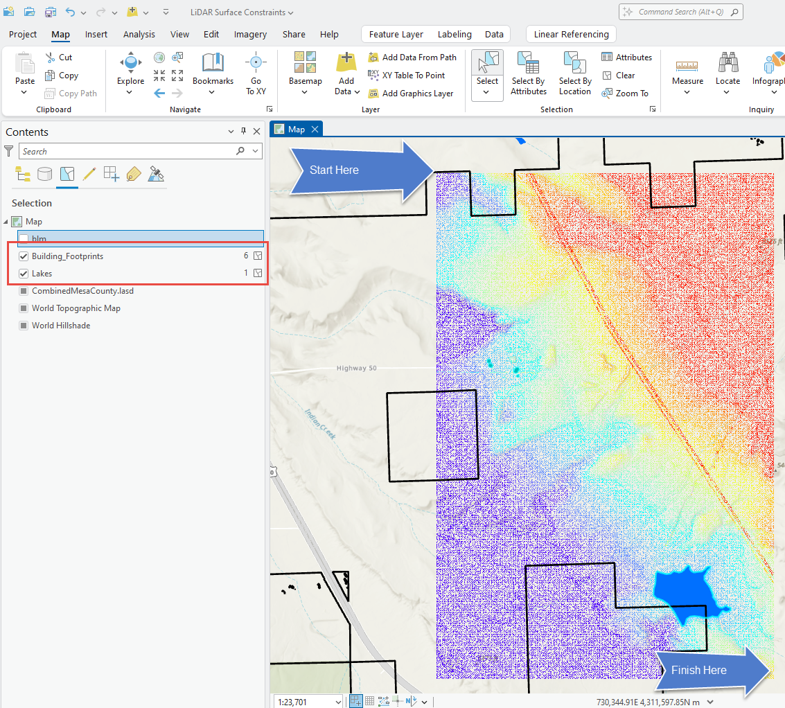
In the map viewer, drag from the upper left corner of all six lidar tiles to the lower right corner of the tiles. One lake and six buildings should be highlighted in cyan and show as selected features in Contents (Figure 23.7).

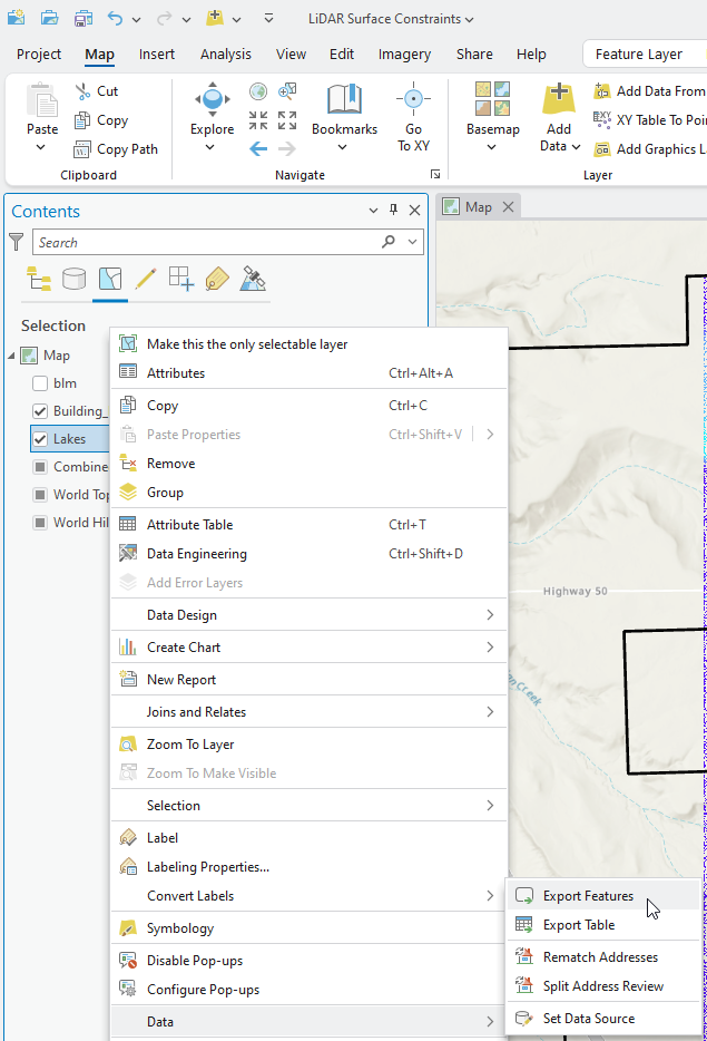
Now let’s create two feature classes: one for the lake and one for the six buildings. Right click on lakes in contents, go to Data > Export Features (Figure 23.8).

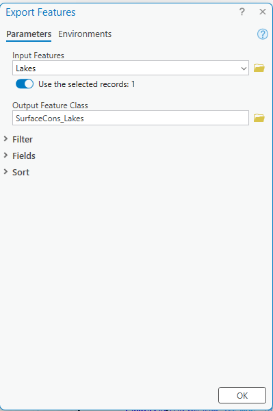
In the Export Features tool name the Output Feature Class “SurfaceCons_Lakes”, leave the defaults for all other parameters and click Ok to run the tool (Figure 23.9).

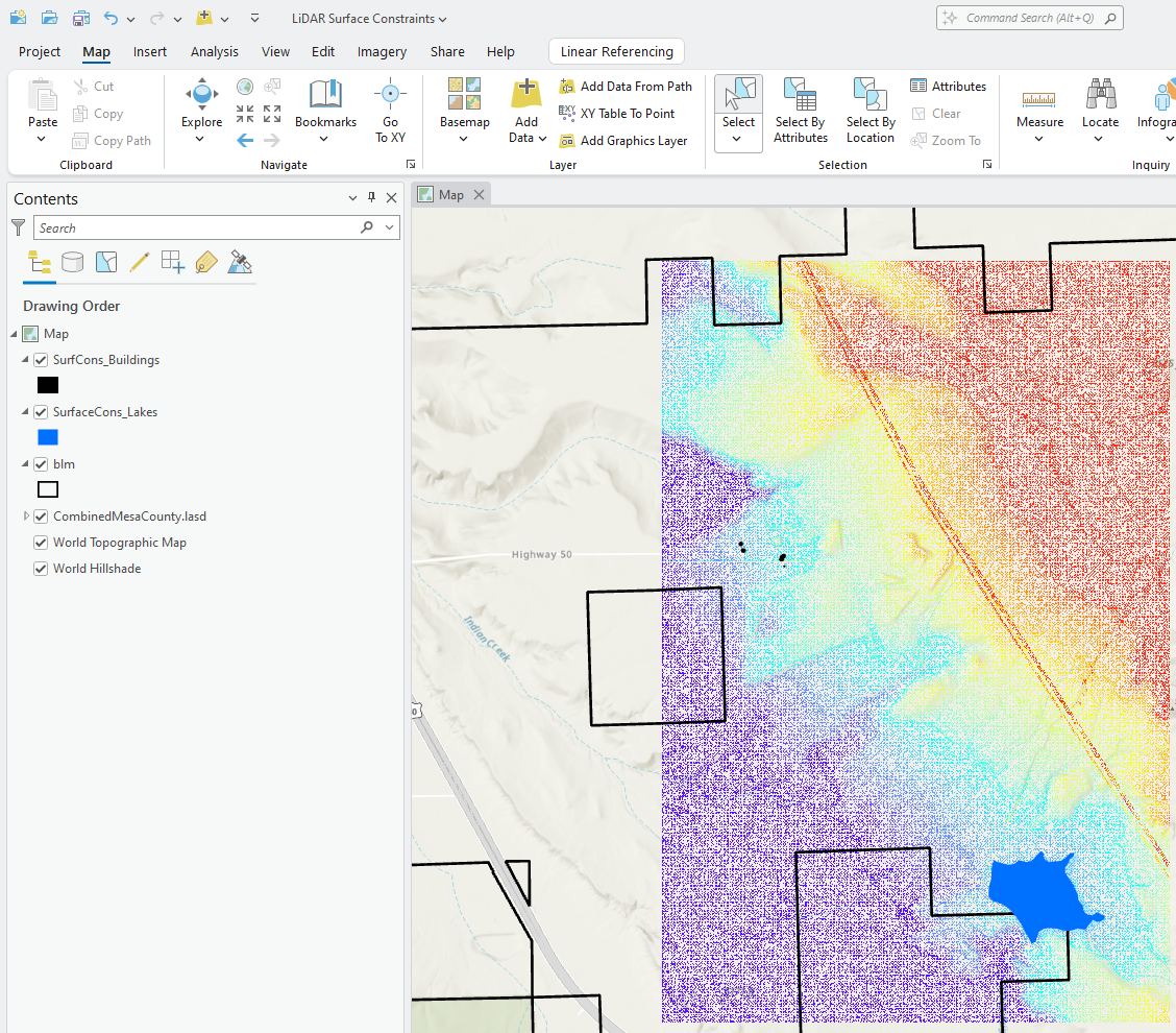
Repeat the process for the Buildings Footprints feature class.  The two new feature classes show in Contents and are displayed in the map window (Figure 23.10).

Turn off the original shapefiles (or remove them) and clear the selection (Clear in the Selection group of the Map tab) (Figure 23.11).

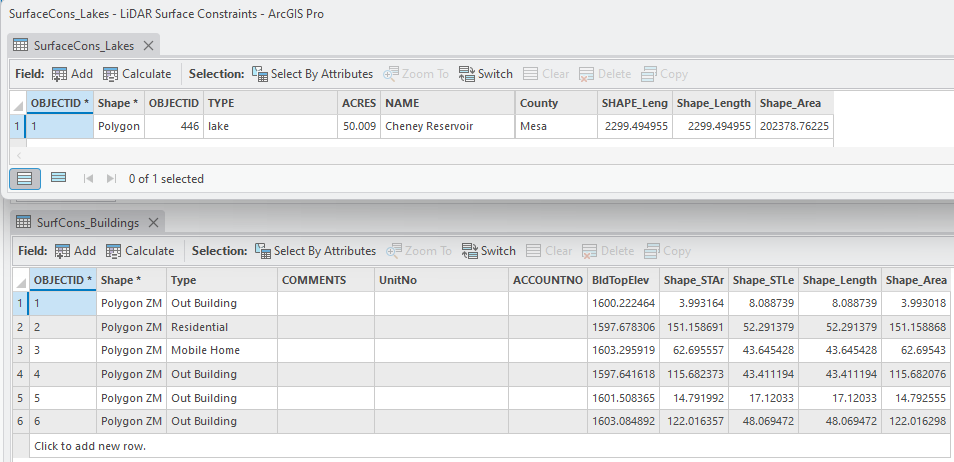
To verify that the only features in the new feature classes are six buildings and one lake, inspect the attribute table for each feature class (Figure 23.12).

These two feature classes can be used as surface constraints. The original shapefiles could have been used but only a few of the features were needed, and by limiting the number of features to the extent of the study area, long processing operation times were reduced.

Understanding Types of Surface Constraints.

Before adding any constraints, understanding the limitations is important.

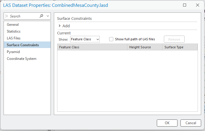
Go to the Catalog Pane or Catalog View, right click on the Combined Mesa Count LAS dataset, open Properties, and choose Surface Constraints (Figure 23.13). None are currently listed.

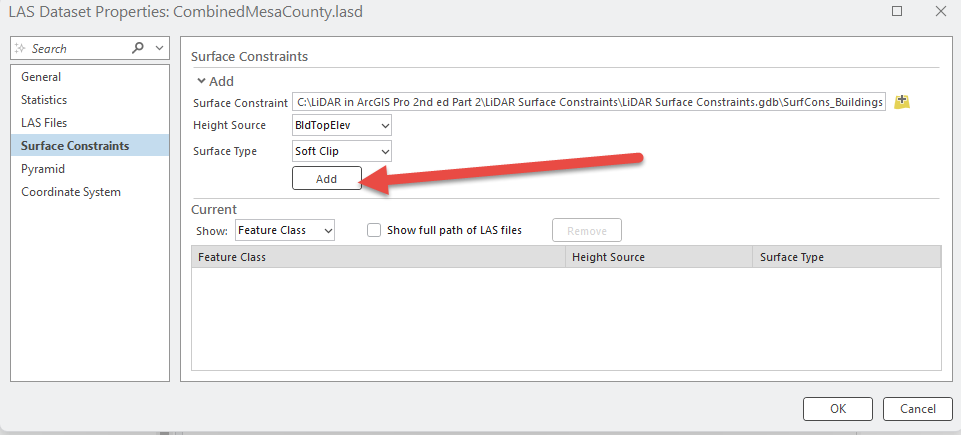
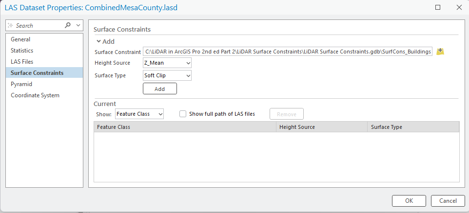
Select Add.  For Surface Constraint, navigate to the location where the new Surface Constraints Building Footprints feature class is saved and select it. Now, the two additional parameters need to be reviewed. Select the down arrow for the Shape field next to Height Source. The options in the drop down are the fields in the attribute table. Figure 23.14

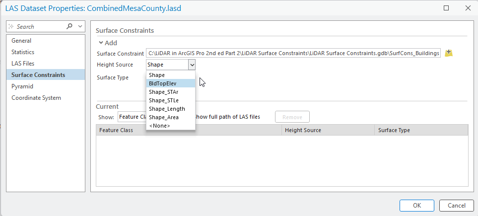
The surface constraint is normally set to use one of the fields in the attribute table as a height variable (elevation above sea level). Choose BldTopElev. When completing a digital elevation model (DEM), eliminating the points representing buildings is appropriate because the top of the building is not normally on the ground (called building top elevation in this attribute table).

Now look at Surface Type. Select the Soft Clip down arrow (Figure 23.15).

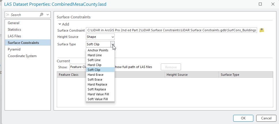
Each one of the parameters listed in Figure 23.15 determines how the surface constraint will be used during geoprocessing and any subsequent operations.

Notice that most of the options start with the words Hard or Soft. Visually, both options create the same image. But the word Hard designates some type of interruption in the surface. Examples of linear features could be a stream, a ridgeline, or the edge of a structure like a building. For a polygon, examples could include building footprints, or edges of a waterbody. The choice of hard or soft as a constraint depends on the project for which you are processing the data.

Anchor Points are elevation points that are never thinned out—this option is only available for single-point data.

Hard Line or Soft Line would be used in instances of breaklines.

Clip and Erase function just like the geoprocessing tools of the same name. Clip will limit data to that inside the boundaries of the polygon. Erase will eliminate points within the polygon.

Replace means that the height value of the lidar points, found within the polygon, will be replaced with the value field you have designated under the Height Source dropdown box.

Choice of Surface Type depends on the project and whether all points are already classified. For example, if all points have been classified and a DEM must be created, using surface constraints can eliminate points classified as buildings, roads, or railways (if a vector feature class exists for each one). Multiple feature classes can be added as surface constraints.

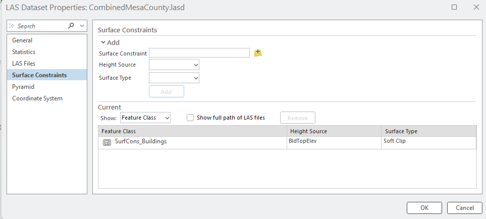
Leave as Soft Clip for now, but these can be changed at will, depending on the project. Please check the appropriate literature or project instructions for determination of the proper Surface Type. When finished, the Surface Constraints dialog should look like Figure 23.16.

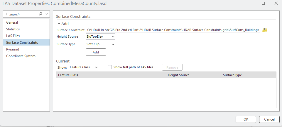
Select Add (Figure 23.17).

The tool processes and the Buildings constraint is added (Figure 23.18).

Close the dialog by clicking on OK (Figure 23.22).

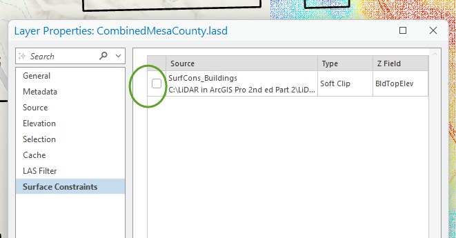
Close the dialog by clicking on OK.  Go back to the Map view.  Then right-click on the LAS dataset in the Contents pane and go to Properties > Surface Constraints. The feature class is listed (Figure 23.19).  The empty box in front of the constraint means that the constraint is not being applied.

What if the attribute table does not have a field (or a useful field) upon which to base a constraint?  For example, the building’s height is in meters and the lidar is in feet.

The buildings file from Mesa County contains the building height, but the height is in meters, whereas the lidar data are in feet.

On the Map tab, click the Explore button then select a building in the map window (Figure 23.20).

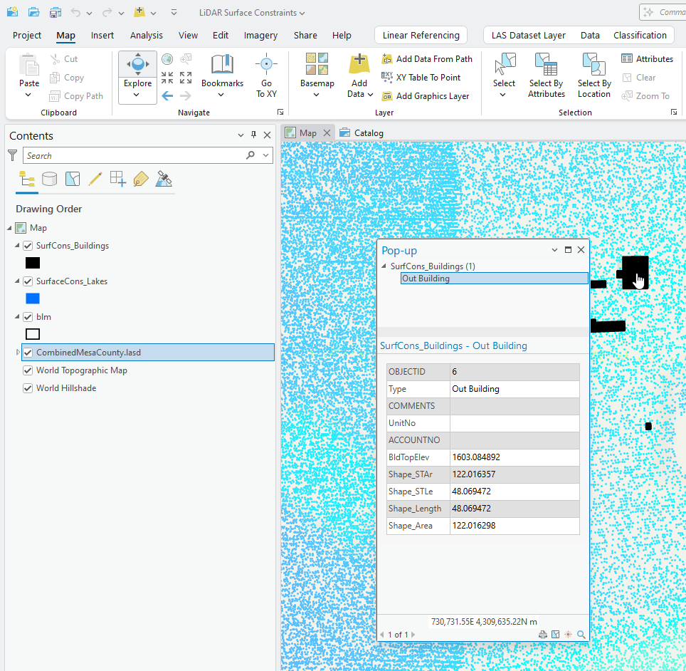
Then check the values for one of the lidar points under the building (Figure 23.21).

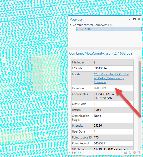
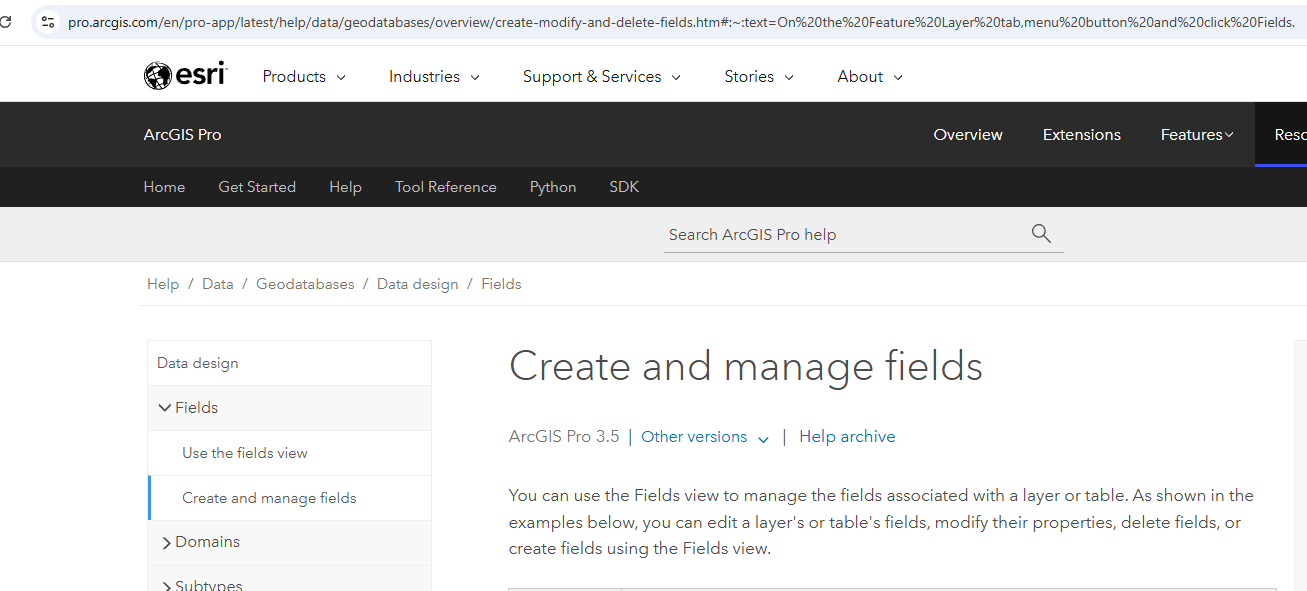
The Building Top Elevation (BldTopElev) and the Z value for the points in the point cloud are similar—1602.309(lidar) and 1603.084892(building shapefile). Although the Pop-up for the lidar says ft, this measurement is in meters. If your height measures are different, then you can add a field in the attribute table and add the measure to be consistent with the elevation in the lidar dataset.  For more information on adding a field within an attribute table, go to ArcGIS Pro Create and Manage Fields and select the Version of ArcGIS Pro that you are using (Figure 23.22).

If there is no height field at all in the buildings’ shapefile you can create a height/elevation field for the buildings using the point cloud. For this demonstration, assume that the building elevation field did not exist in this Mesa County buildings shapefile.

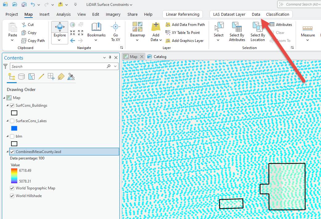
In the Contents, select the .lasd file and the LAS Dataset Layer menu and two associated tabs appear (Figure 23.23).

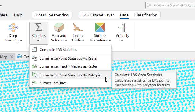
Choose the Data tab, click the down arrow under Statistics, and choose Summarize Point Statistics by Polygon (Figure 23.24).

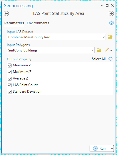
The LAS Point Statistics by Area Geoprocessing tool opens (Figure 23.25). The Input LAS Dataset field automatically populates. Choose Surface Cons_Buildings from the dropdown arrow for Input Polygons. The Output Property is the new field that is going to populate in the attribute table of the SurfaceCons_Buildings feature class. For this example, check all the Output Property boxes.

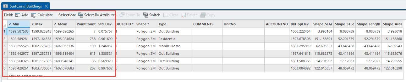
All the new fields are now in the attribute table—the maximum value of all points contained within the boundaries of each building polygon, the minimum value, the mean, how many points were used and the standard deviation. ArcGIS Pro® automatically recognized the Z values as meters (Figure 23.26).

Now that the vector feature class used for surface constraints has different fields that can be used, how has the Surface Constraint field in the LAS dataset changed?

Go to the Catalog Pane or Catalog View and open Properties for the LAS dataset. Select Surface Constraints. Select the feature class present and click Remove (Figure 23.27).

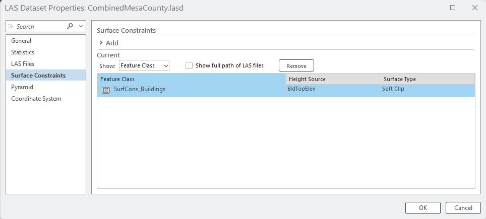
Click Add and add SurfaceCons_Buildings again and choose the new field Z Mean for the Height Source (Figure 23.28).

Again, which Surface Type should be used? Consult the appropriate literature pertaining to the analysis being completed.

What if a water body is the feature used for a surface constraint, and the attributes do not include a height (or a water depth value)—recall the Lakes attribute table. Go back to Map view, right click on Lakes > Zoom to Layer. The lake does have some points within its boundaries (Figure 23.43).

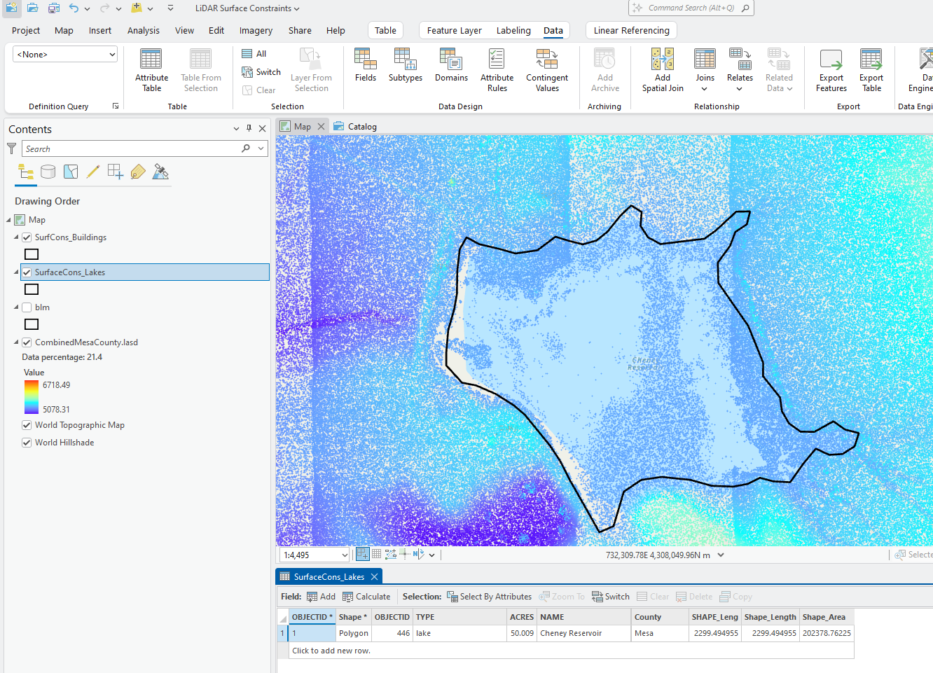
As done with Buildings, values could be extracted but water depth is difficult to determine from a lidar point cloud because clear and/or deep water absorbs lidar, and the points displayed within the polygon could be reflected from surface features, debris or sediment. Compare the lidar point cloud and the Google Earth® image of the lake in Figure 23.30. Some surface features are clearly visible, including some vegetation.

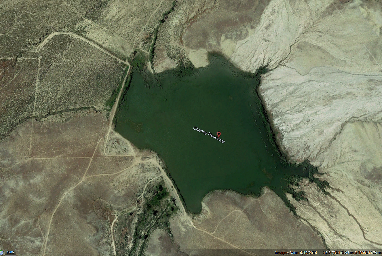
A field could be added if the water depth values were known. According to the Colorado Birding Trail^[1], the Cheney Reservoir is a shallow irrigation lake, and no depth documentation is provided.

So how to proceed with no depth/elevation information? To eliminate points within the boundaries of the lake from the analysis, use a Hard Erase for Surface Type and none for Height Source. These will be demonstrated in the next chapter.

From Catalog View or the Catalog Pane, add the Lakes  feature class as a Hard Erase  Surface Type (Figure 23.31).

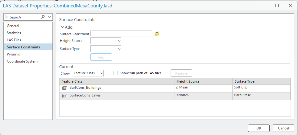
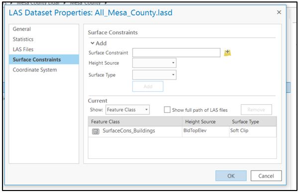
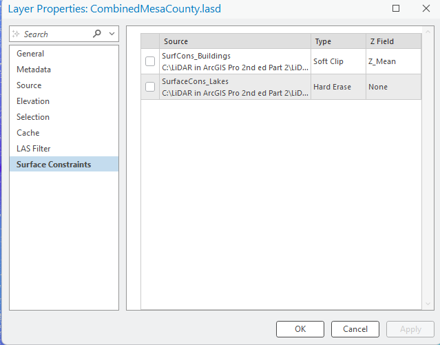
From Map view, check the properties of the .lasd file to verify that both of the feature classes are listed under Properties > Surface Constraints (Figure 23.46).

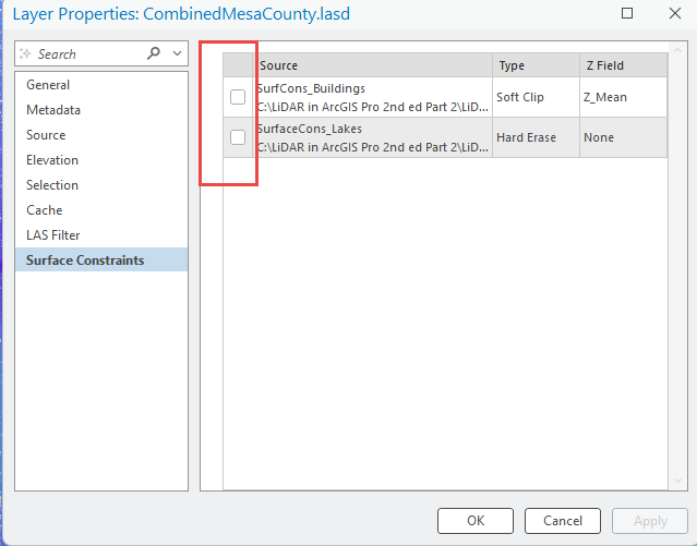
As a final note, once surface constraints have been added to a LAS dataset, they need not be removed if they are not going to be used in analysis or processing. When surface constraints are to be applied, select the constraint to be used by checking its checkbox (Figure 23.33) before running any geoprocessing tools.

The next chapter will demonstrate the results when surface constraints are applied and when they are not applied.