Chapter 22. Creating a Digital Elevation Model
Introduction
Classifying Lidar Points (Chapters 18-21) explains the processes employed to classify points in a point cloud. This chapter will demonstrate the process of creating a digital elevation model and a digital surface model and provide examples of the settings used to create these data models. This chapter also reviews additional raster operations available from lidar data.
What is the difference between a digital elevation model and a digital surface model? A digital elevation model (DEM) is the elevation of the surface of the Earth with nothing on it. A DEM is commonly known as a bare earth model. A digital surface model (DSM) is a raster rendering of the first returns of lidar data[1]. As noted in Chapter 7. Locating Lidar Data, a first return can be bare earth, the top of a building or the top leaf of a tree, as examples. When creating a digital elevation model from lidar points, all ground points must be classified first because only ground points are used.
Open a new map scene and add the San Luis Valley dataset. Be sure to display ground points only (Figure 22.1), all classifications created in the last few chapters have been retained.
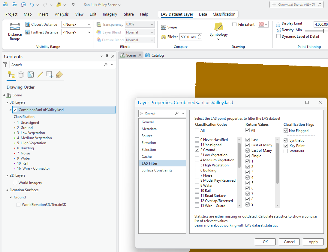
These data are displayed as elevation data. But remember, this is a symbolization of a lidar point cloud only, it is not a digital elevation model. A digital elevation model (DEM) is a raster dataset. A conversion tool is necessary to create a DEM from a lidar dataset.
Digital Elevation Model Examples
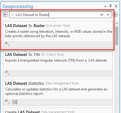
Under the Analysis tab on the ribbon, choose Tools and search for “LAS Dataset to Raster” (Figure 22.2). As you are searching, ArcGIS Pro® provides options that match your search below the search box. Alternatively, go to Toolboxes and expand Conversion Tools > LAS.
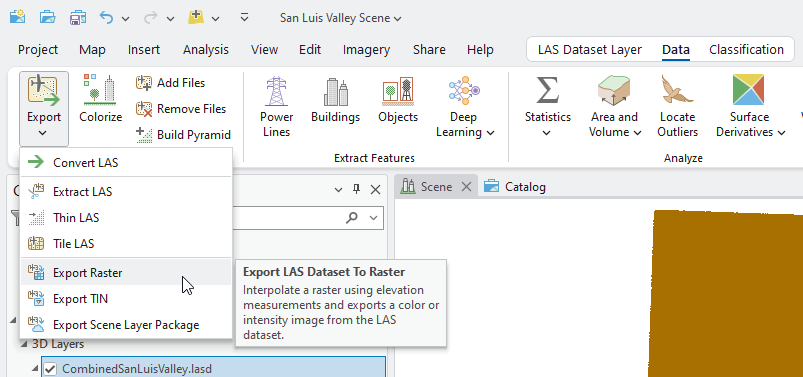
There is also a shortcut icon found under the LAS Dataset Layer > Data > Export drop-down menu—Raster, which also opens the Export LAS Dataset to Raster tool (Figure 22.3).
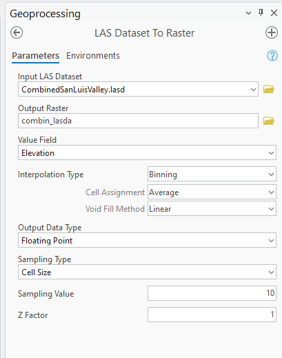
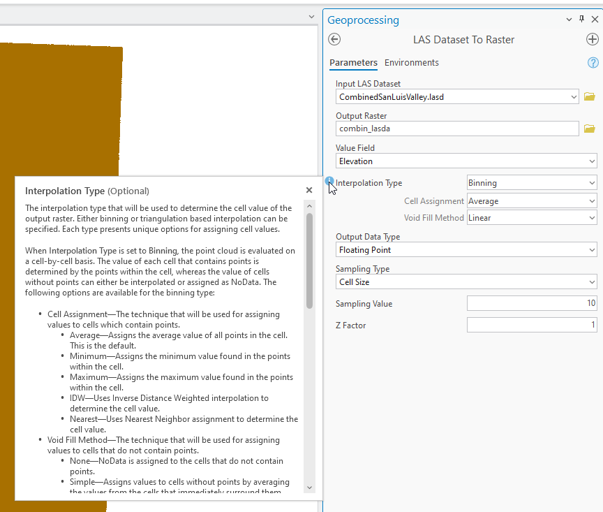
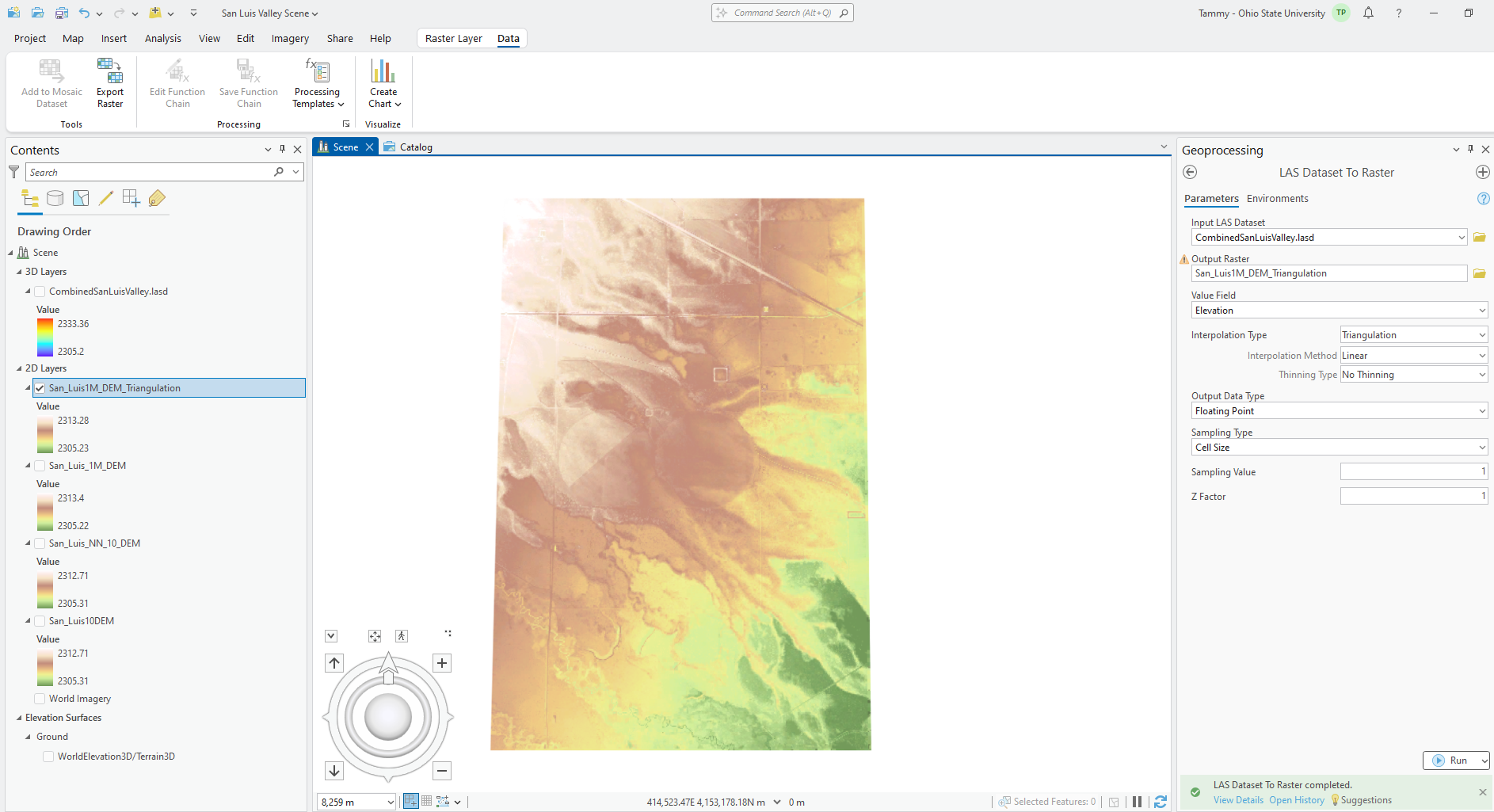
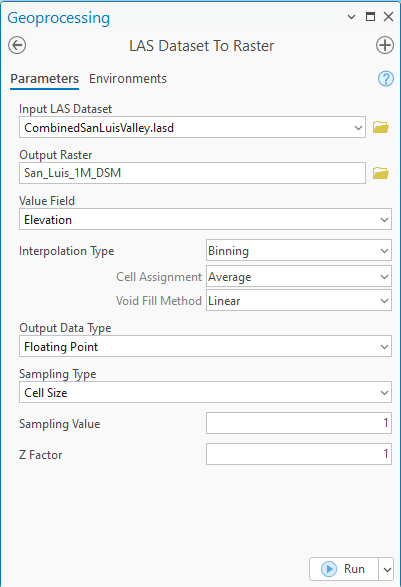
See Figure 22.4 to follow these steps. Interpolation Type will be discussed last.
- Choose the Input LAS Dataset from the drop-down list. (The dataset does not need to be in the project. If it is not, use the folder at the end of the line to navigate to the computer’s folder where the .lasd dataset is located.)
- Under Output Raster, name the new file. Name it something meaningful to help identify it in the future. For example, San_Luis10Dem (for 10-meter dem).
- The Value Field is elevation.
- Output Data Type is Floating Point (the other option is Integer). Use Floating Point as elevation values are not always whole numbers.
- Sampling Type for a DEM, use Cell Size.
- Sampling Value is the resolution for the Cell Size of the new raster. Leave this as 10, other values will be explored later. Remember the unit of measurement from prior chapters? It is expressed in meters! So, the resolution will be 10 meters.
- Z Factor leave as 1. If this is changed, the vertical differences will be exaggerated. Only change this value if creating a dataset for display purposes only and exaggeration of vertical differences is useful. Do not use a setting other than 1 when creating a DEM for analysis.
For Interpolation Type (Figure 22.5), the defaults are Binning, Average and Linear. The choice of settings for these three depends on many factors, including a corporate preference, a government’s preference, or the specific project for which the DEM is being created. For example, a different method may be chosen for delineating a watershed for a forested area (which must begin with a DEM) as opposed to a watershed in an urban area. Please consult the appropriate academic literature for assistance with this decision-making process. It is important that you read all the information on the Interpolation Type available through the information icon within ArcGIS Pro – use the scroll bar to review.
For this initial example of the tool, leave the default values for all fields. To initiate the DEM creation, click Run to execute the tool (Figure 22.6).
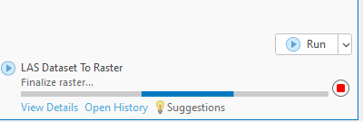
A progress bar displays at the bottom of the geoprocessing window (Figure 22.7).
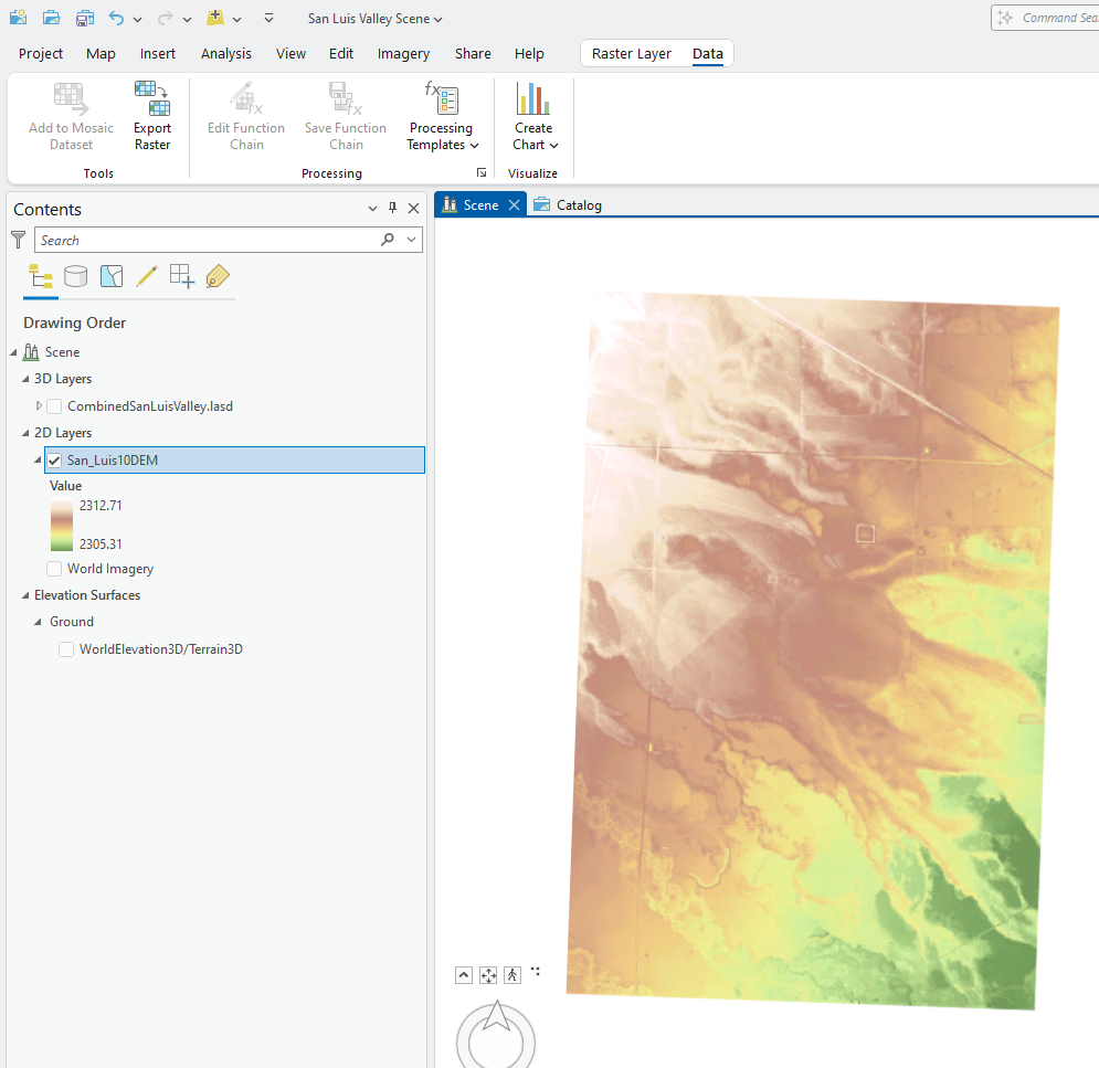
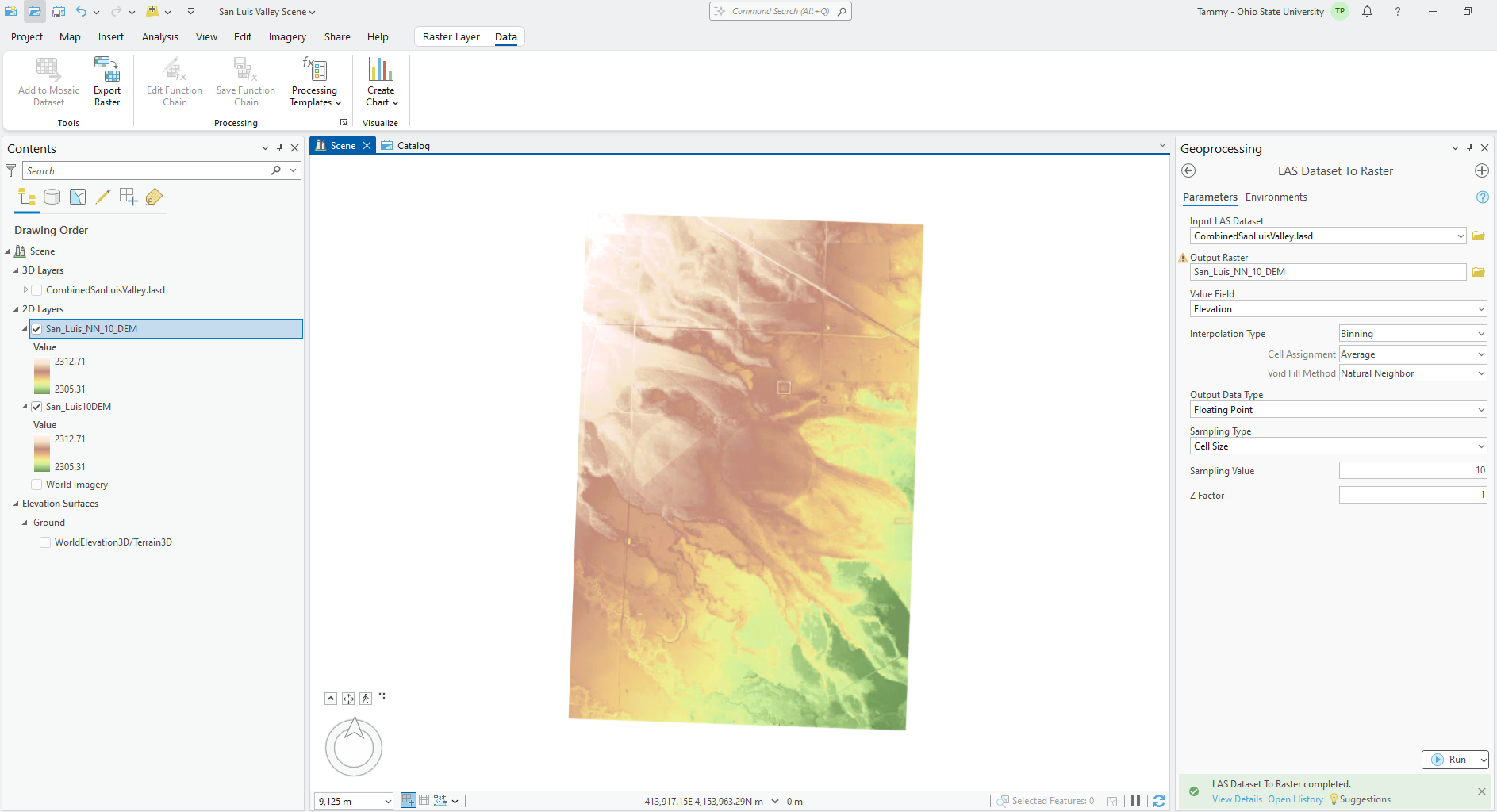
When finished, the DEM is automatically added to contents and the map viewer and displays in stretched symbology under the lidar point cloud. Turn the LAS dataset off and change the elevation symbology to Elevation #4 (Figure 22.8).
Run the tool again but use Natural Neighbor as the Void Fill Method (Figure 22.9). Be sure to change the symbology to Elevation #4.
There is very little difference between the two DEMS from just changing this one setting—Linear versus Natural Neighbor. Constructing a DEM with a 10-meter resolution from a lidar point cloud with less than a 1-meter point density does provide a difference in the resulting DEMs.
Change the Sampling Value to 1 (1-meter resolution) (Figure 22.10). Leave the defaults for all other values.
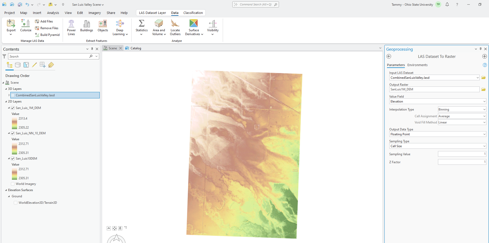
The range of values for the resulting DEM is slightly different from the prior two DEMs. Zoom in to the area shown in Figure 22.11.
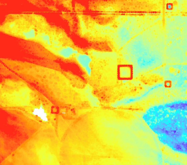
The greatest difference when creating a DEM from lidar data is the resolution. Comparing the 1-meter DEM (Figure 22.12) to either of the 10-Meter DEMs (Figure 22.13), the finer resolution at 1 meter has more distinct features.
Whether to create a 10-meter DEM or a 1-meter DEM depends on the purpose of the DEM but also on the point density. The ability to acquire lidar at greater pulse densities (more pulses per unit area or less ground distance between pulses) allows for finer resolution DEMs
Run the tool once more using Triangulation as the Interpolation Type and 1-meter Sampling Value. Notice when this setting was changed, Void Fill Method changed to Thinning Type. (Remember to read the literature and the tool information in ArcGIS Pro.) Again, there is a slight change in the range of values (Figure 22.14).
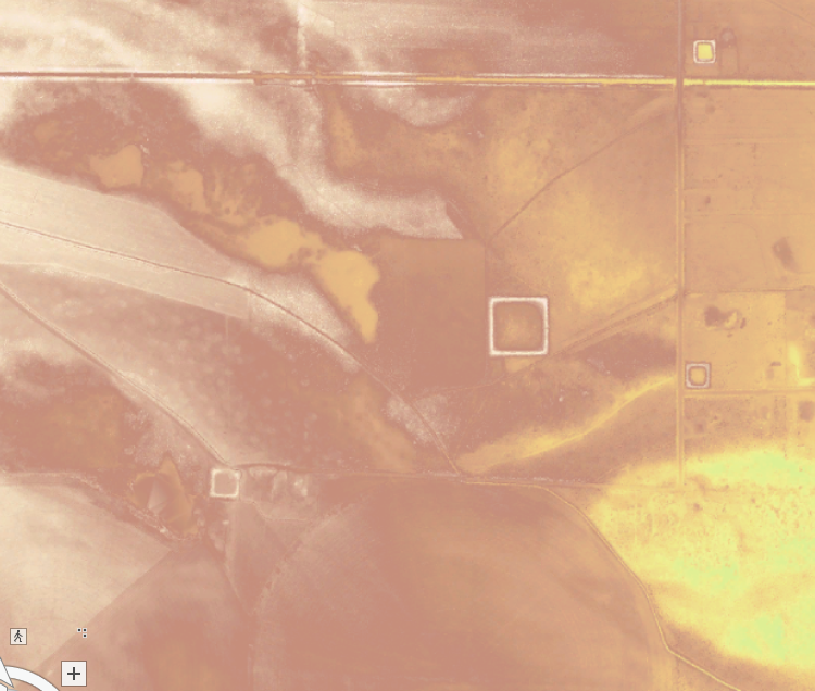
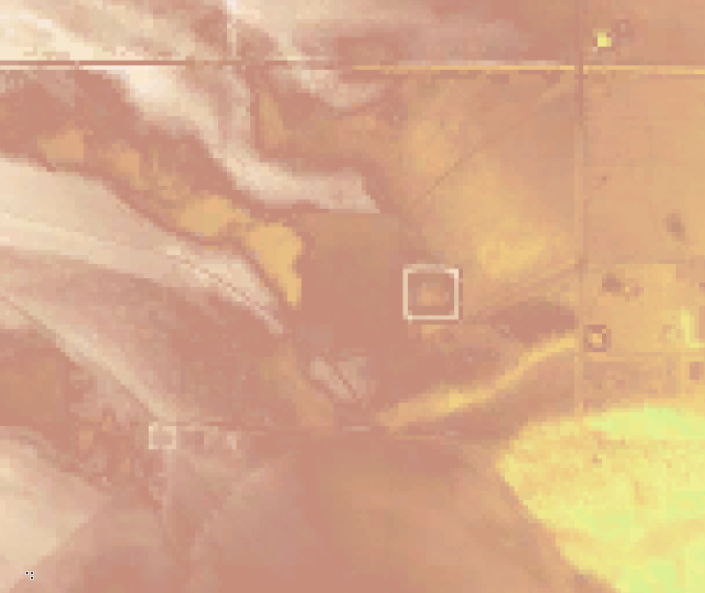
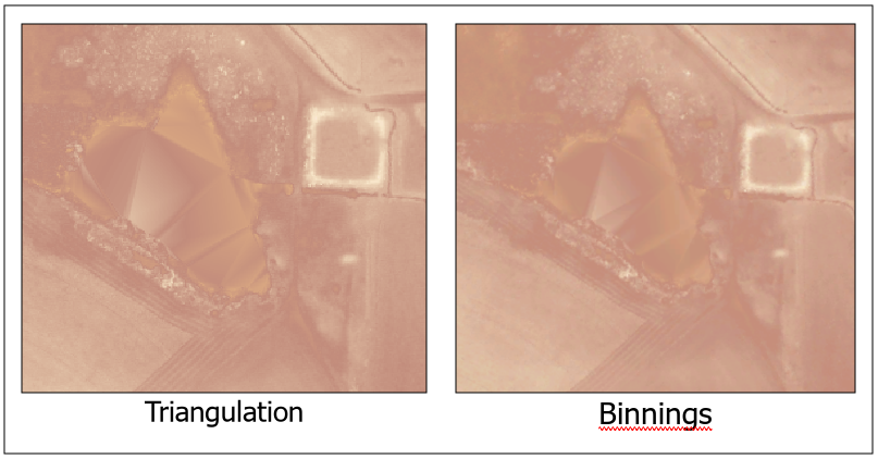
Zoom further in to the lake (Figure 22.15), the main difference appears to be interpolation across missing values. Please note these results are specific to this dataset. Other datasets may produce different results.
Digital Surface Model Examples
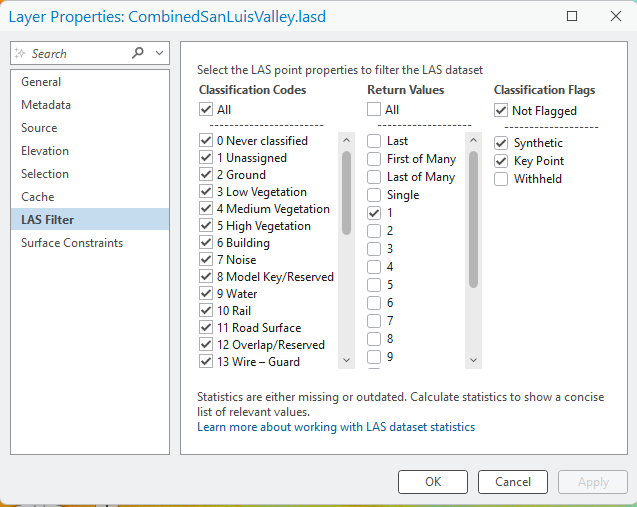
Now let’s create a digital surface model (DSM). First, set the LAS Filter to the first return (Figure 22.16). The classification code does not matter, it will only use first returns, no matter what class code the point is assigned.
Open the LAS Dataset to Raster tool, leave all settings default except for Sampling Value, set it to 1 . Be sure to name Output Raster appropriately (Figure 22.17).
The results are much different from the raster generated for the Digital Elevation Model. Buildings are also visible (Figure 22.18).
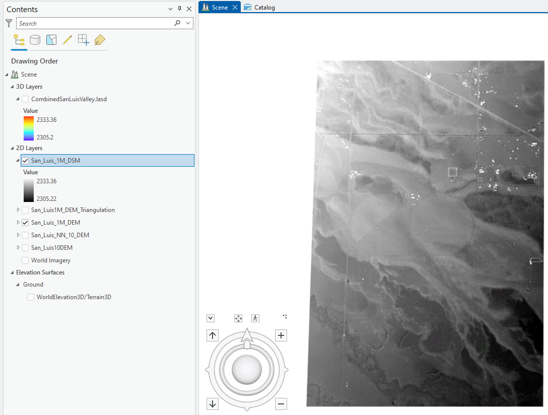
Figure 22.19 shows the 1-meter DSM and 1-meter DEM side-by-side (Binning method).
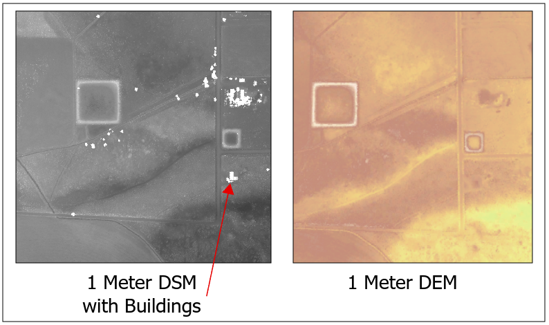
Which to use (DEM versus DSM) depends on the project. If delineating a watershed, a DEM is used because first returns from a building top or treetop are not appropriate for a watershed delineation. Refer to academic literature for the appropriate uses for each type of raster.
Using the Lidar Generated DEM to Create other Data Types
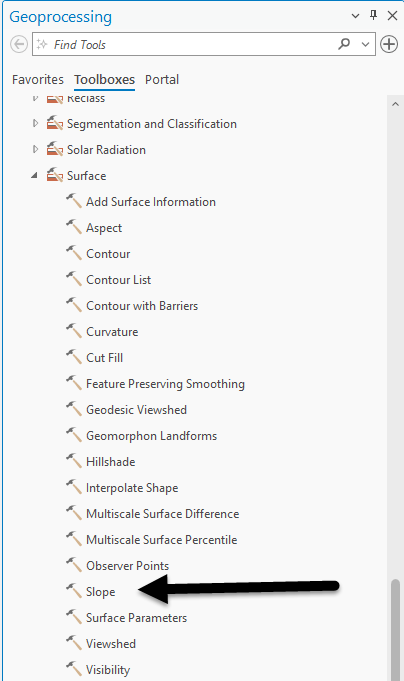
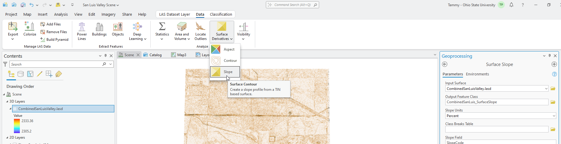
Using a DEM created from the lidar data, other datasets can be constructed. Among them, a slope file can be created using the Spatial Analysis > Surface > Slope tool (Figure 22.20). Please note, ensure your organization’s administrator has authorized the Spatial Analysis Extension to you as a user of ArcGIS Pro®.
Use the 1-meter DEM(Binnings) to create a Slope. Use Percent Rise and not Degrees for the calculation (Figure 22.21). Once the slope file is created, symbology can be changed as with other files.
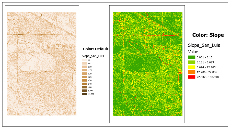
Slope can also be created directly from the LAS dataset. Use the shortcut icon under LAS Dataset Layer > Data > Surface Derivatives drop-down menu (Figure 22.20).
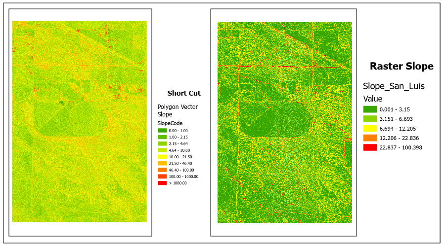
Please note that this tool does take a bit longer to run and it creates vector data, not raster. It appears that the tool did not run correctly because it seems to be mostly gray—this is polygon vector data, and each category has a gray outline around it. Go to Symbology and change the outline color around all the polygons to no color (Figure 22.23). Except for the number of classes and the color, the slope values are the same for any specific location.
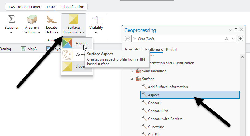
Aspect can be created from a DEM using spatial analyst tools or directly from the LAS dataset under 3D Analyst Tools or using the shortcut under LAS Dataset Layer > Data > Surface Derivatives. (Figure 22.24).
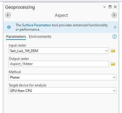
Use the Geoprocessing tool Aspect. The Input raster is the 1-meter DEM. Use the default setting, Planar, and be sure to name the output raster appropriately. (Figure 22.25)
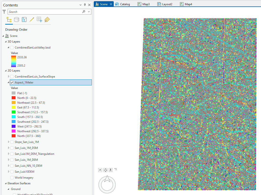
The results (Figure 22.26) are similar to the aspect symbology completed in Chapter 16. Lidar Symbology.
What is the difference? Chapter 16. Lidar Symbology provided an overview of symbology; no new dataset was created. The file created here can be used to complete a watershed delineation, for example. Symbology cannot be used as an input to another geoprocessing operation.
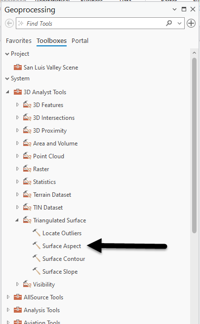
Now under 3D Analyst Tools, choose Triangulated Surface > Surface Aspect (Figure 22.27). Be sure to set the LAS Filter to Ground points. The Aspect shortcut can also be used to open the tool.
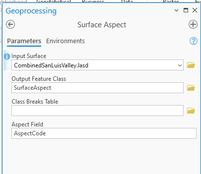
The Input Surface is the LAS dataset. Name the Output Feature Class appropriately—something memorable and related to the new dataset. Surface Aspect also includes an input for a Class Breaks Table (optional). (Figure 22.28).
Why include a Class Breaks Table? Without a Class Breaks Table, normal definitions for aspect values, the range of azimuthal degrees that correspond to a cardinal direction (Figure 22.29) are assigned.
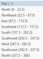
A Class Breaks Table might be necessary when more specific delineations of aspect are required, such as North Northeast or West Southwest, in addition to the delineations identified in Figure 22.29. A Class Breaks Table is not used in this chapter, so leave that field blank.
Once the tool is completed is as shown in Figure 22.28, select Run.
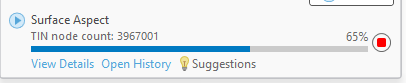
Because the tool is processing all points classified as ground (~12,000,000 points in this example), it takes a bit longer to execute. Several status messages will display during processing. Figure 22.30 is an example of one.
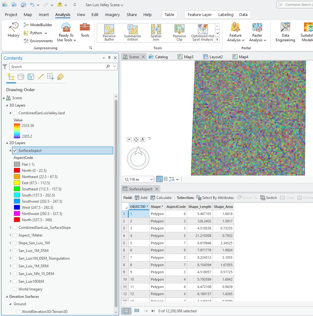
The Surface Aspect tool creates a feature class (polygon) with an attribute table (Figure 22.31). Over eleven million polygons were created, thus the reason for the lengthy processing time. Again, if the resulting feature class appears all gray, change the outline color for all polygons to no color.
The processing time for the Surface Aspect tool was lengthy. The process for the Spatial Analyst Aspect tool required two steps. Which is better? It depends on the project. One resultant file was a feature class, the other a raster. So, which is best for the project? This is the question to be answered using appropriate literature or project parameters.
There are other tools available now that new rasters have been created. This Chapter will not review them.
The final two chapters cover setting and utilizing surface constraints.
- From the United States Geological Survey at https://www.usgs.gov/faqs/what-difference-between-a-dem-and-a-dsm. ↵
