Chapter 21. Classifying Points Using Geoprocessing Tools
The previous three chapters introduced classification codes, interactive classification, and geoprocessing tools for classifying points in a lidar point cloud. This chapter demonstrates four of the geoprocessing tools—Classify Ground points, Classify by Height, Reassign Classification, and Feature Proximity.
As a reminder, the ASPRS Classification codes are:
| Classification Value | Classification Description |
|---|---|
| 0 | Never classified |
| 1 | Unassigned |
| 2 | Ground |
| 3 | Low Vegetation |
| 4 | Medium Vegetation |
| 5 | High Vegetation |
| 6 | Building |
| 7 | Low Noise |
| 8 | Reserved |
| 9 | Water |
| 10 | Rail |
| 11 | Road Surface |
| 12 | Reserved |
| 13 | Wire – Guard (Shield) |
| 14 | Wire – Conductor (Phase) |
| 15 | Transmission Tower |
| 16 | Wire-Structure Connector (Insulator) |
| 17 | Bridge Deck |
| 18 | High Noise |
| 19-63 | Reserved |
| 64-255 | User Definable |
Either open the project created in Chapter 19. Interactive Classification or create a new local scene and add the San Luis Valley dataset.
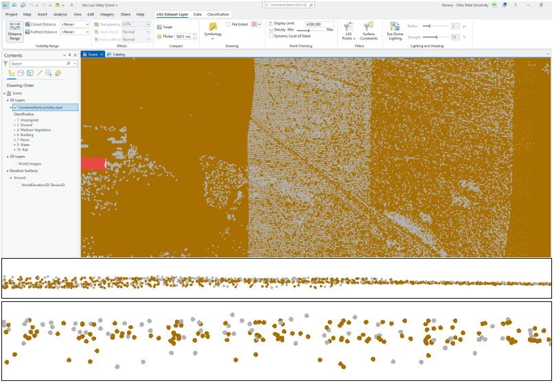
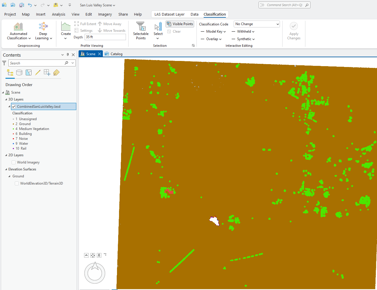
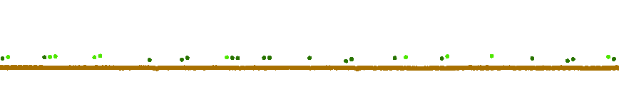
Let’s start with Classify Ground. Some, not all, ground points are classified. Zoom in to the location visible in Figure 21.1, just east of the buildings and vegetation that were interactively classified in Chapter 19. Interactive Classification and create a profile view (Figure 21.1). A variety of unassigned points are found in this region, many that look like ground points. Let’s practice on this limited extent to see how the tool operates.
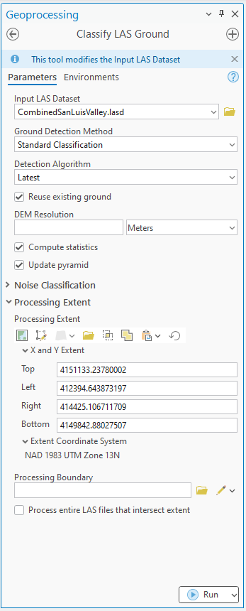
Leave the profile view open and open the Classify Ground tool. Leave all default parameters except check the boxes for Reuse Existing Ground and use Current Display Extent. When Current Display Extent is chosen, the coordinates of the area are entered into the tool automatically (Figure 21.2). Run the tool.
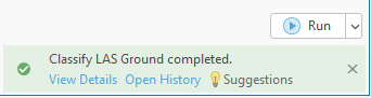
When the tool finishes, a completed message displays at the bottom (Figure 21.3),
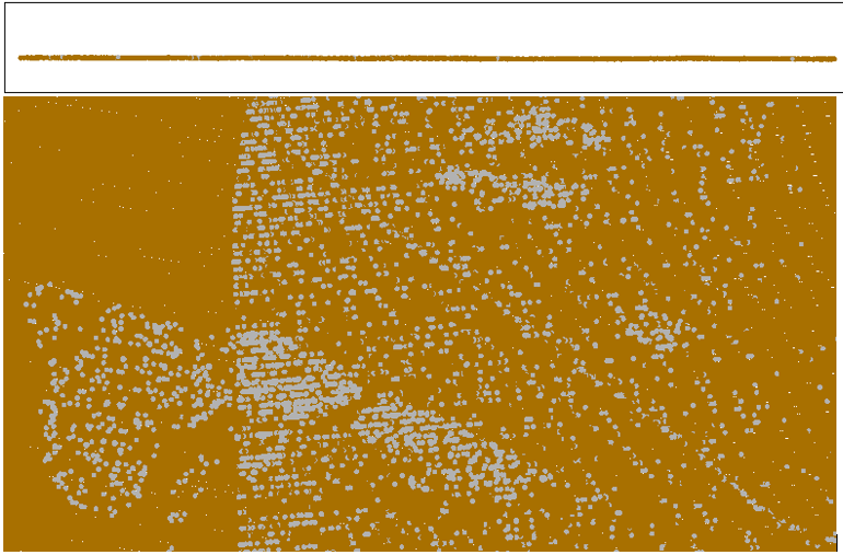
and for points now identified as ground, the point symbology has changed (Figure 21.4).
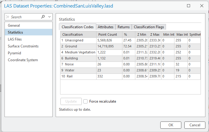
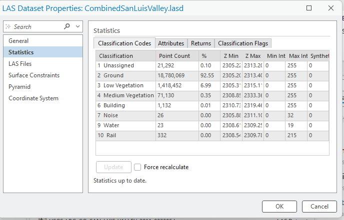
Go to Properties in Catalog View and check the Statistics (Figure 21.5). Because the compute statistics box was checked in the tool, the statistics are up to date.
Zoom out and run the tool one more time but for a greater extent (Figure 21.6).
When the tool finishes, the number of unassigned points is significantly less, while the number of ground points has increased (Figure 21.7).
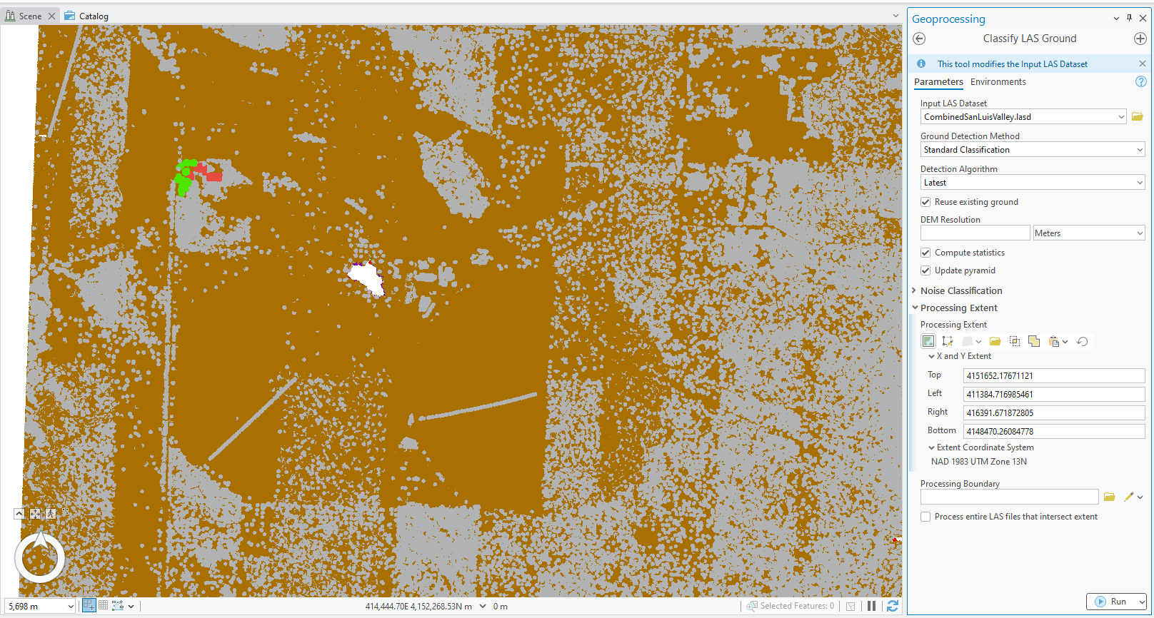
If comfortable with this tool and the settings, go ahead and process the entire dataset for ground points. Leave all settings as default with the exception of checking the box for Reuse Existing Ground. Please note that since the extent includes a larger region, the tool takes longer to run.
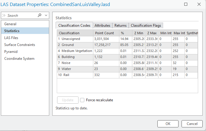
Figure 21.8 shows the statistics after the entire dataset has been processed using the Classify Ground tool. A significant number of unassigned points still exist.
Now, let’s run the Classify by Height tool. Zoom in to the region from Chapter 19. Interactive Classification where buildings and medium vegetation (trees) were identified (Figure 21.9).
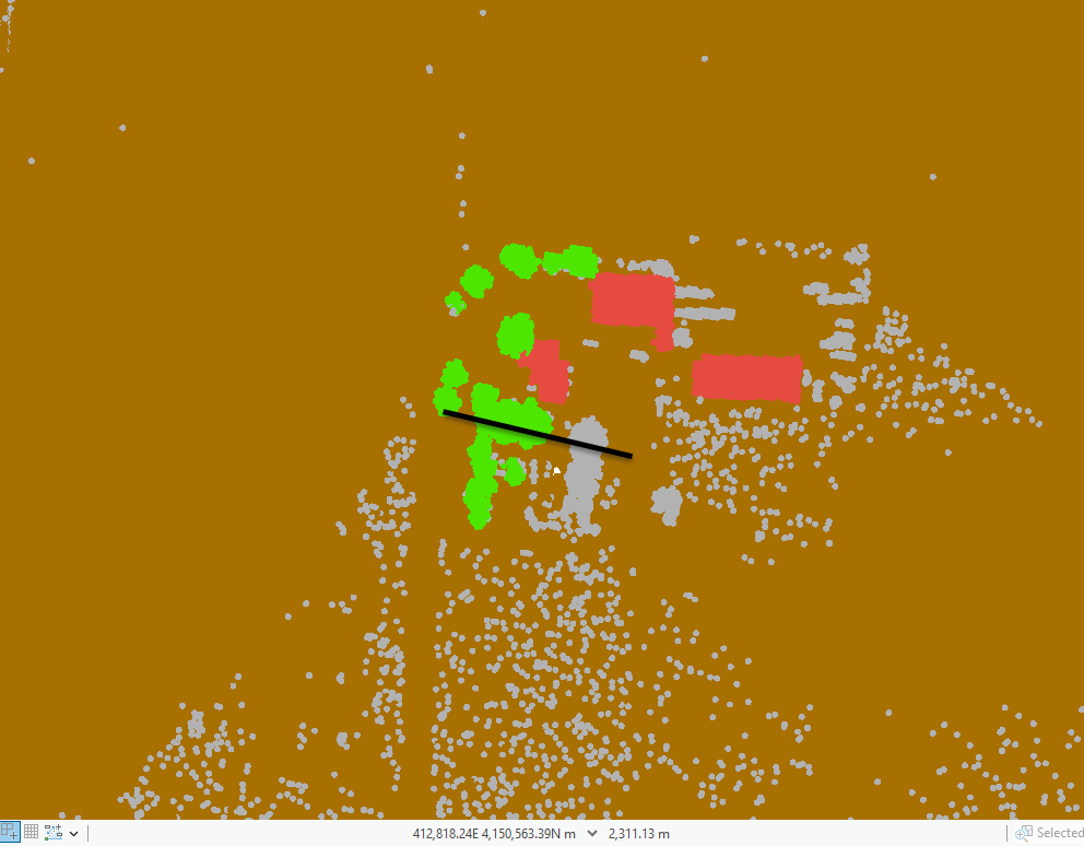
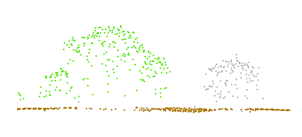
Using the black line in Figure 21.9 as a guide, create a profile view across that location (Figure 21.10).
Be careful with the depth setting so you don’t also include the roof of the building to the North. Then, we first need to determine the distances above ground for the range of points for a specific classification.
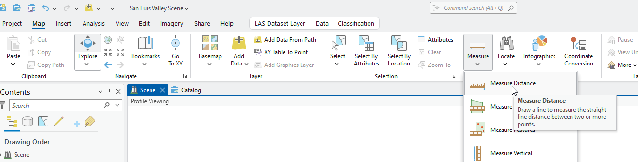
To measure the distances from ground to the various locations in the profile, you can go to the Map tab and click on the Measure tool and Measure Distance between points, but this tool is extremely difficult to use in profile view. (Figure 21.11).
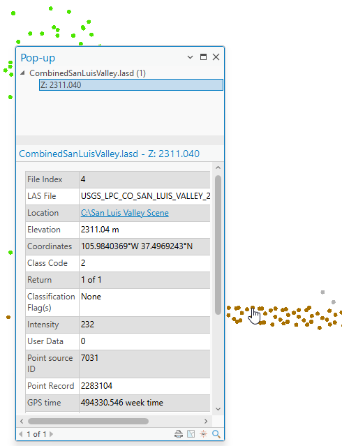
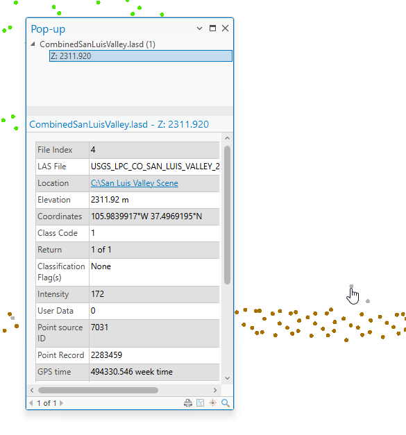
An easier way to calculate the distances is just clicking on a specific point and the pop-up gives you the elevation value for that point. Zoom in to a ground point and click on it. Figure 21.12 shows the pop-up for a ground point.
Now choose one of the unassigned points that is closest to the ground (Figure 21.13).
Now check the values for one of the lower points on the tree canopy (Figure 21.14) and one of the highest points on the tree canopy (Figure 21.15).
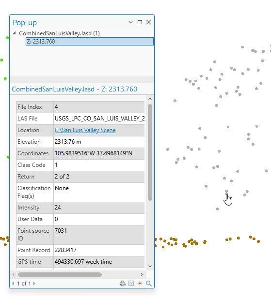
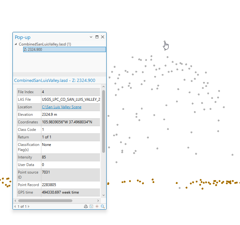
The distance between a ground point and the unassigned is .88 meters (2311.92 – 2311.04), from ground to lower tree canopy is 2.72 meters (2313.76 – 2311.04), and from ground to highest tree canopy is 13.96 (2324.9 – 2311.04). Please note that your values may be different depending on which points you choose.
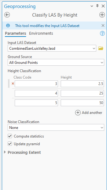
Now open the Classify by Height tool. Remember from Chapter 20. Introducing Geoprocessing Tools for Classification that the values in height are the maximum value that will be used to determine the classification, e.g. low vegetation (3) is ground up to 5 meters, medium vegetation (4) is over 5 up to 25 meters, and high vegetation (5) is over 25 to 50 meters. Based on the previous measurements, change the values of low vegetation to 2.5 meters and medium vegetation to 15 meters. Leave high vegetation as the default. Also, leave Ground Source as All Ground Points, Noise Classification as None and the Processing Extent as Default. Click Run to process the entire dataset (Figure 21.16).
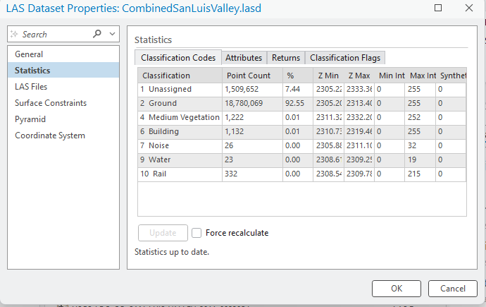
The number of unassigned points is significantly reduced, and vegetation values have been assigned throughout the entire dataset for those range of distance values (Figure 21.17). Figure 21.18 shows the updated statistics.
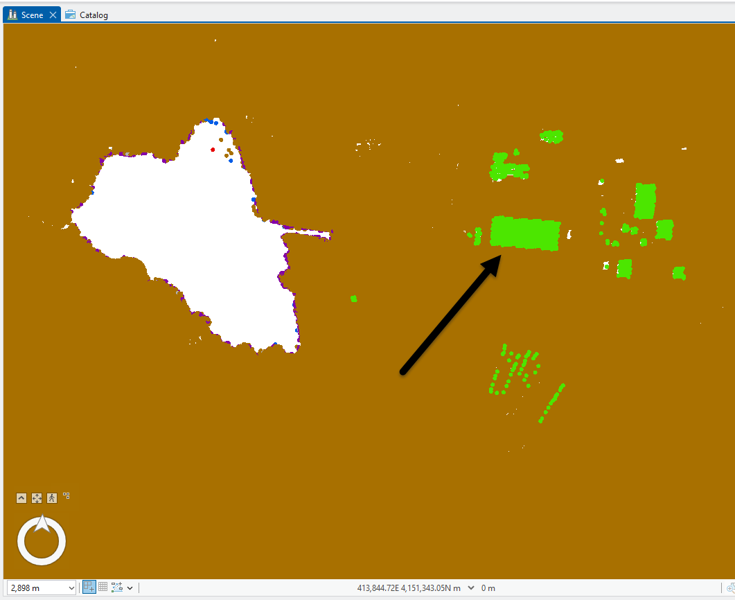
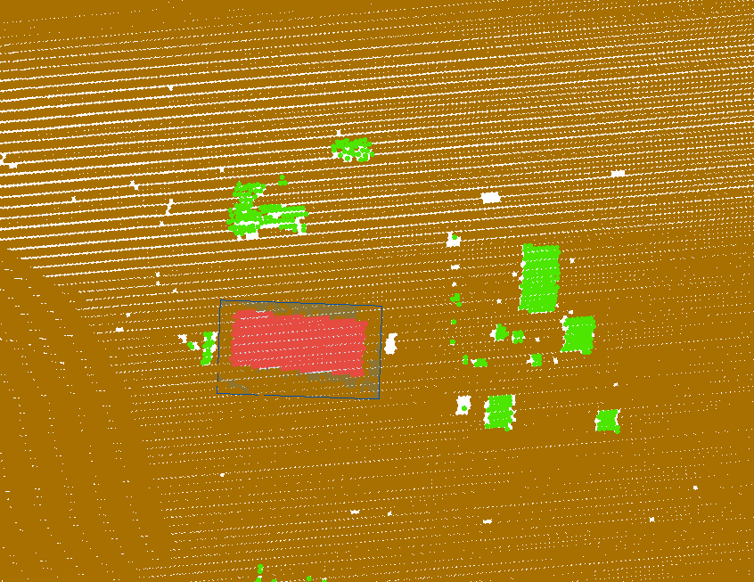
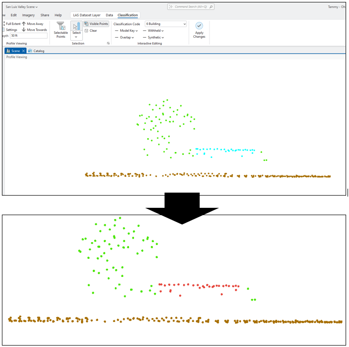
Zoom in to the area just to the east of the lake (Figure 21.19). In some instances, vegetation values, both low and medium vegetation, have been assigned to buildings or other features. Please note only the unassigned points were assigned values by the Classify by Height tool. In Chapter 19. Interactive Classification, with interactive processing, only a few buildings points were classified. Now, let’s see how to correct a misclassification.
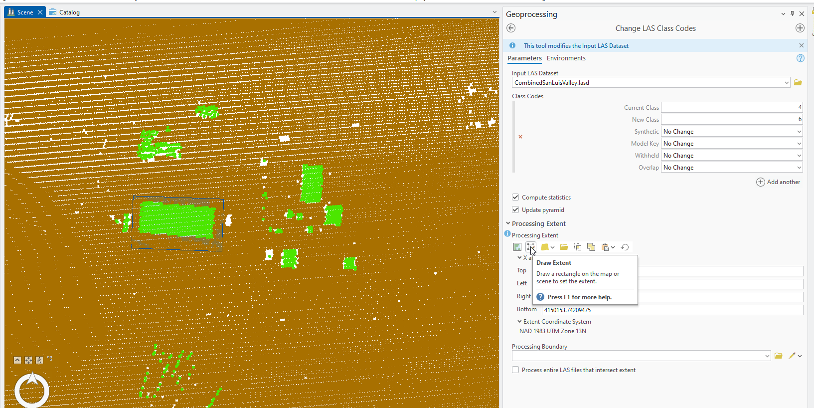
Select Reassign Classification to open the Change LAS Class Codes tool. Enter the values shown in Figure 21.20. Current Class is 4 (medium vegetation) and New Class is 6 (building). Expand Processing Extent and click on the Draw Extent tool and use this tool to draw a polygon around one of the buildings. Double click to end the drawing (Figure 21.20). Then Run the tool.
Results are shown in Figure 21.21. Only the points for that specific building should have changed.
You can use this tool to continue to correct these misassigned points, even grabbing two buildings if there are no actual vegetation points between the two (Figure 21.22).
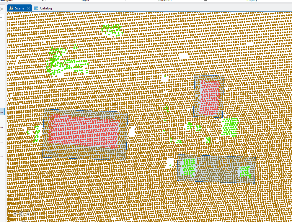
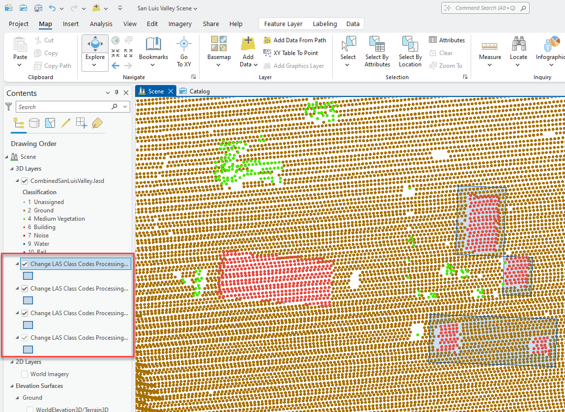
As you use the Draw Extent tool, it adds a new polygon layer in Contents for each of the polygons that you draw. The polygons will stay in the map viewer (Figure 21.23). You can either turn them off in Contents or remove them.
Let’s correct those points just north of the largest building. Zoom in and create a profile view (Figure 21.24). Some are building/roof and some are medium vegetation. It would be difficult to use an overhead view in the prior steps to reassign some of this vegetation as a building (roof).
Use interactive classification within this profile view to change the classification codes appropriately (Figure 21.25). Refer to Chapter 19. Interactive Classification if a refresher is needed on interactive classification.
For one final example using one of the Proximity to Features tool, recall from Chapter 20, a feature class is needed to use the 2D tool, with the current version of ArcGIS Pro®, it cannot be created from this tool. So, we will demonstrate the Set Class Code Using 3D Proximity to Features tool.
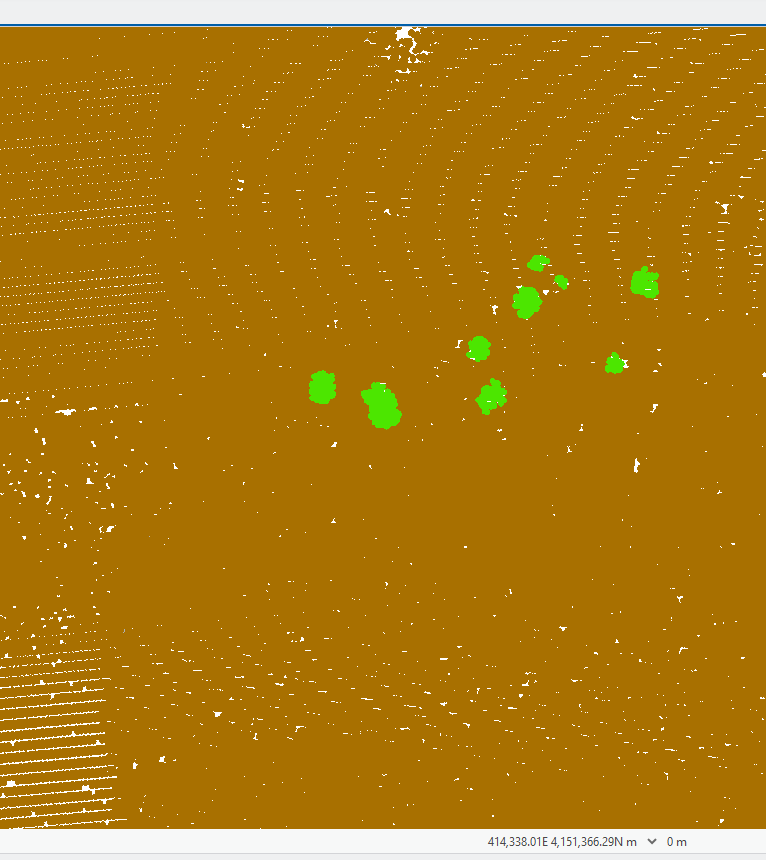
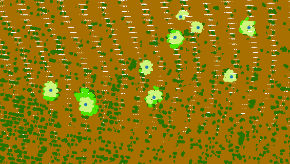
First, zoom in to the trees seen in Figure 21.26, these are slightly northeast of the location we were just using.
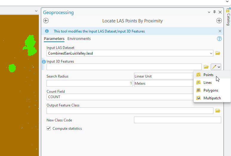
Open the Set Class Code Using 3D Proximity to Features tool, which allows for creation of a feature class (Figure 21.27). Click on the pencil icon at the end of Input 3D Features and select Points. The Points drawing tool opens. This tool will allow adding a point to each of the trees.
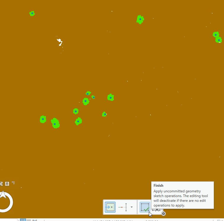
Click the center of each tree to add a point. Once all the points shown are added, select Finish (Figure 21.28).
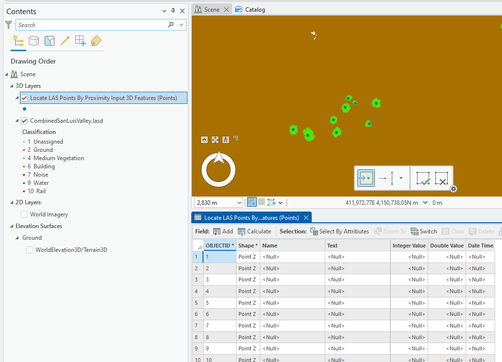
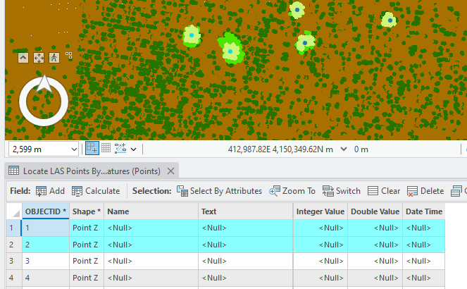
In Contents a new file named (by default) is listed—Locate LAS Points by Proximity Input 3D Features (Points). Open the attribute table for this new file—there are the features representing each of the tree points just created (Figure 21.29). Close the table.
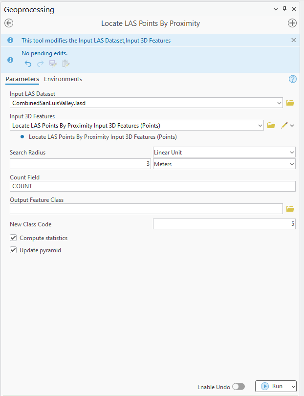
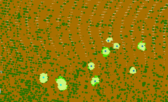
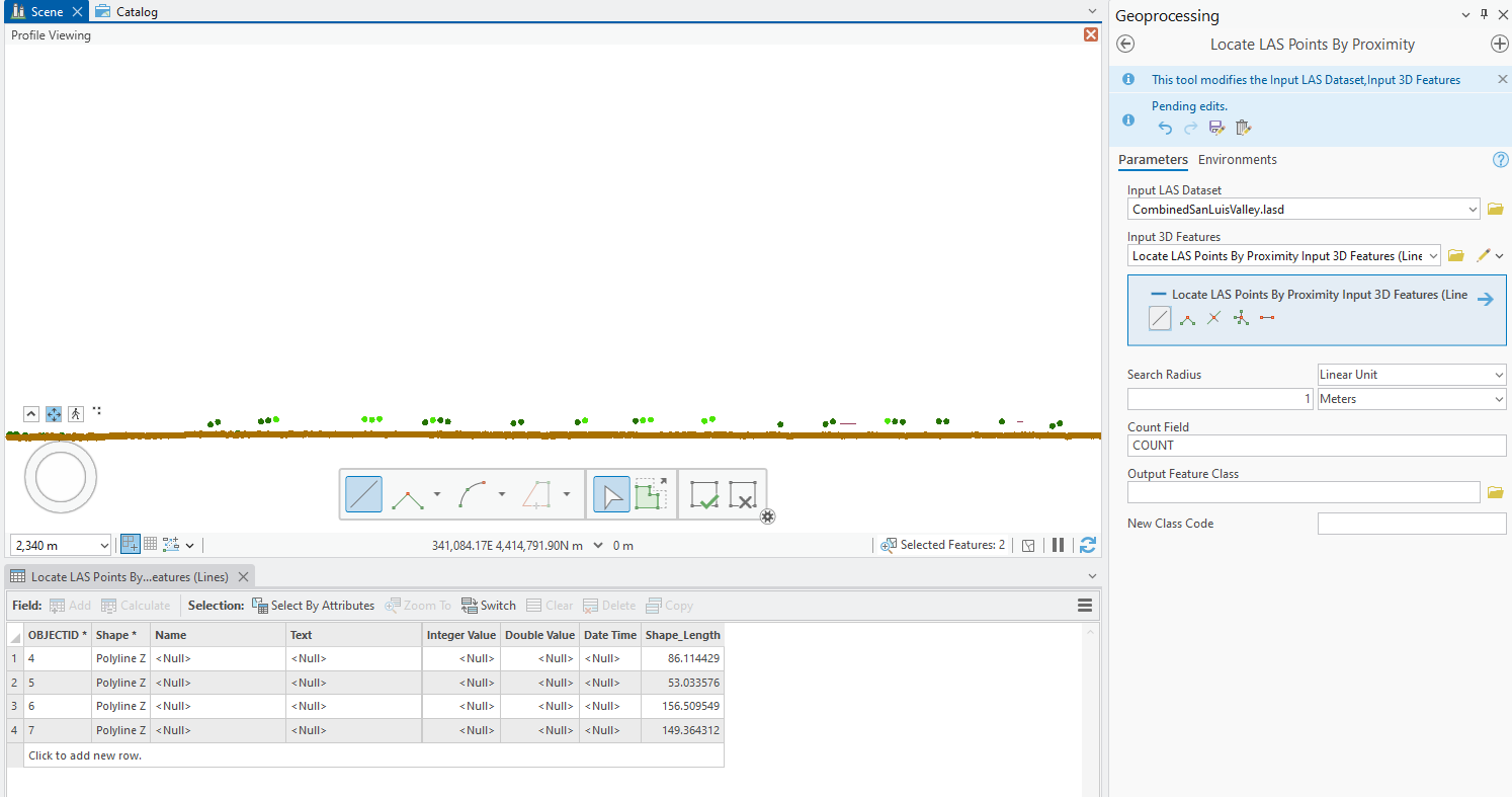
Now open the 3D Proximity tool. The Input Feature Class, the one just created, is now populated within the tool. Use a Search Radius of 3 (any lidar point within 3 meters of the point feature class will be recoded) and change the New Class code to 5 (high vegetation – these trees may not qualify as high vegetation, but this code is being used here as an example of the tool’s operation) (Figure 21.30). Click Run.
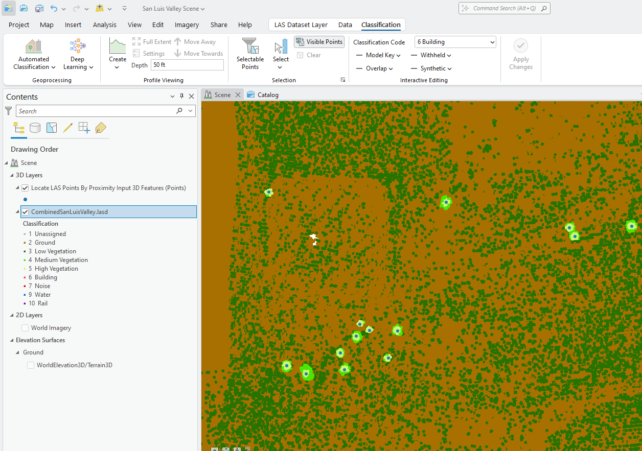
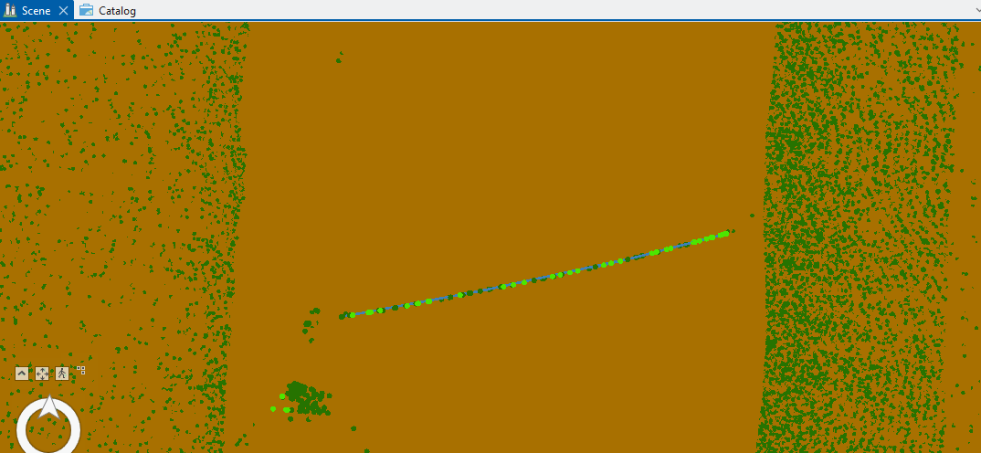
The trees, lidar points within 3 meters of the feature points, are now coded as high vegetation (Figure 21.31). The points are not symmetrical around the feature points because this is a 3D scene, and points are not necessarily an equal distance from each other.
There are still a considerable number of points that could be reclassified, so run the tool again using the same parameters except increase the Search Radius to 4 meters (Figure 21.32).
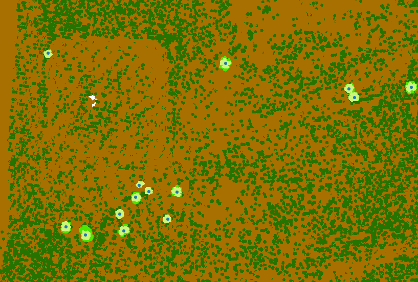
The resulting coverage is much better for many of the trees but the two on the left still has several lidar points coded as medium vegetation (Figure 21.33).
Open the attribute table for the Locate LAS Points by Proximity Input 3D Features (Points) feature class. Select the feature points that corresponds to these two trees (hold down Ctrl to select the 2nd one)(Figure 21.34).
Within the 3D Proximity tool, increase the Search Radius to 6 meters and run the tool again. The tool will apply changes to the selected features only—the trees selected in the feature class (Figure 21.35). Compare the classification on the trees from Figure 21.34 to Figure 21.35, only those two trees that were selected have additional points classified as 5 – High Vegetation.
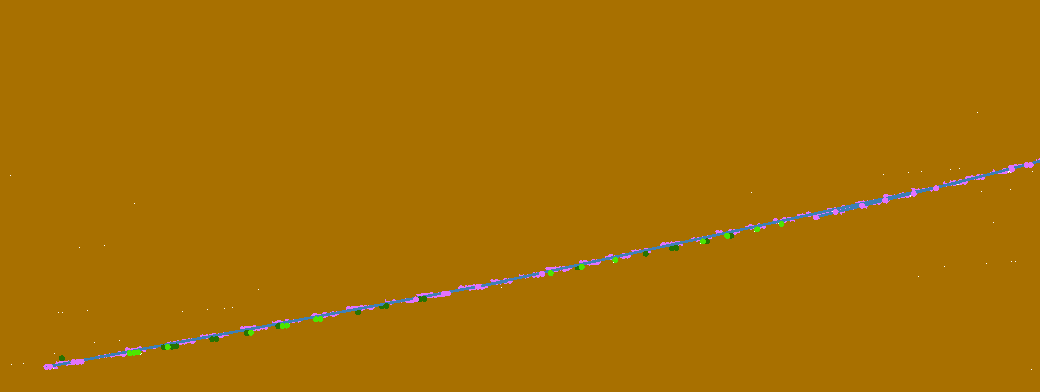
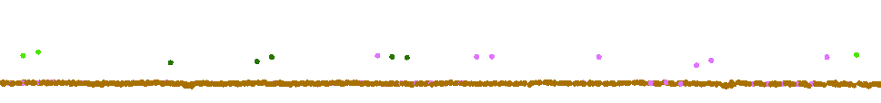
Let’s do one more example. Remember the pivot irrigation line (Figure 21.36)? (If you are having problems finding it, it is located just south of the Lake in Figure 21.19.)
Create a profile view (Figure 21.37).
Open the 3D Proximity tool and create a line feature. A line feature is a linear connection between nodes—a node is created with each mouse click. Create a line over the pivot irrigation equipment, getting as close to each lidar point as possible and creating as many nodes as needed. Once complete, click Finish in the drawing toolbar (Figure 21.43).
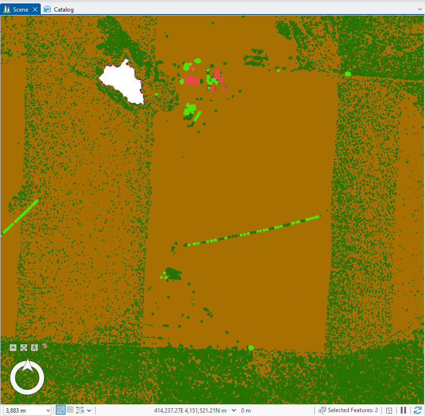
Close the Profile View and the line feature has been created (Figure 21.39).
Open the 2D Proximity tool. Use the new feature class as the Input Feature Class, add a Buffer Distance of 0.5, and since no class code currently exists for this type of feature, use 16 (one of the wire codes). Click Run (Figure 21.40).
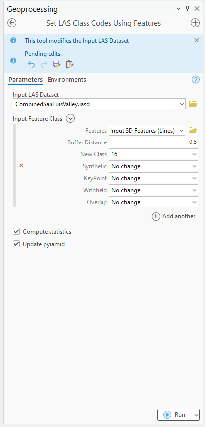
Figure 21.41 displays the result. Some points still remain low vegetation, and it appears some ground points were reclassified. It may be necessary to turn off the line feature class in Contents to better view the results.
In profile view (Figure 21.42), it is evident that not all points were changed but some ground points were inadvertently changed. The buffer distance could have been set to 1 meter but, in all likelihood, more ground points would have been changed.
As with other tools demonstrated in this chapter, interactive classification can be very useful to fix small misclassifications (Figure 21.43).

When classifying lidar point clouds, there is no one classification tool that will process all points at one time, so multiple classification methods must be used.
Continue to work on classifications to try to classify as many as the unassigned points as possible. When creating a digital elevation model, ground points will be used, so in order to be as accurate as possible when creating the model, all ground point classification should be finished.
This ends the chapters on classifications. The next chapter will demonstrate the creation of a digital elevation model (DEM) from a lidar point cloud.
