Chapter 20. Introducing Geoprocessing Tools for Classification
Chapter 18. Introduction to Classification introduced point classification and classification schemes. Chapter 19. Interactive Classification demonstrated classifying points interactively. This chapter will introduce the geoprocessing tools available for classification and Chapter 21. Classifying Points Using Geoprocessing Tools will demonstrate some of the tools.
The ASPRS LAS classification codes listed in Table 1, including classification descriptions, are updated by the ASPRS regularly. Thus, please check the ASRPS website regularly at https://www.asprs.org/.
| Classification Value | Classification Description |
|---|---|
| 0 | Never classified |
| 1 | Unassigned |
| 2 | Ground |
| 3 | Low Vegetation |
| 4 | Medium Vegetation |
| 5 | High Vegetation |
| 6 | Building |
| 7 | Low Noise |
| 8 | Reserved |
| 9 | Water |
| 10 | Rail |
| 11 | Road Surface |
| 12 | Reserved |
| 13 | Wire – Guard (Shield) |
| 14 | Wire – Conductor (Phase) |
| 15 | Transmission Tower |
| 16 | Wire-Structure Connector (Insulator) |
| 17 | Bridge Deck |
| 18 | High Noise |
| 19-63 | Reserved |
| 64-255 | User Definable |
This chapter does not demonstrate the use of geoprocessing tools. It introduces the tools available for classification and provides instructions on the many decisions that must be made when classifying lidar points.
Open the project created in the last chapter or create a new local scene and add the San Luis Valley LAS dataset. Any classifications completed in the previous chapter will appear in the San Luis Valley dataset even if a new project is created.
Go to the Analysis tab and open Tools. Many of the Geoprocessing tools for classification of lidar points are listed under 3D Analyst Tools, so select Toolboxes and search for “3D Analyst.” and then expand the Point Cloud > Classification. But there are many other tools to process LAS datasets, located in different toolboxes, as seen in Figure 20.1. In this chapter, we are only discussing the classification tools.
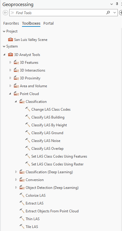
Alternatively, ArcGIS Pro® provides shortcut icons that will open these tools.
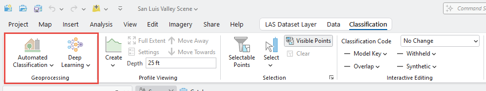
Go to the Classification tab. On the left side of the ribbon are two different classification options in the Geoprocessing group—Automated Classification and Deep Learning (Figure 20.2).
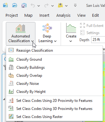
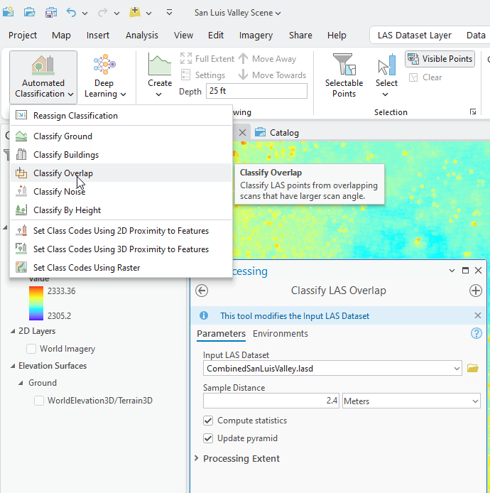
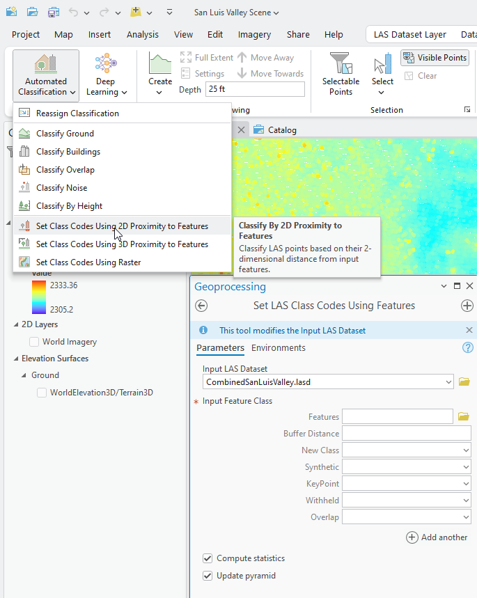
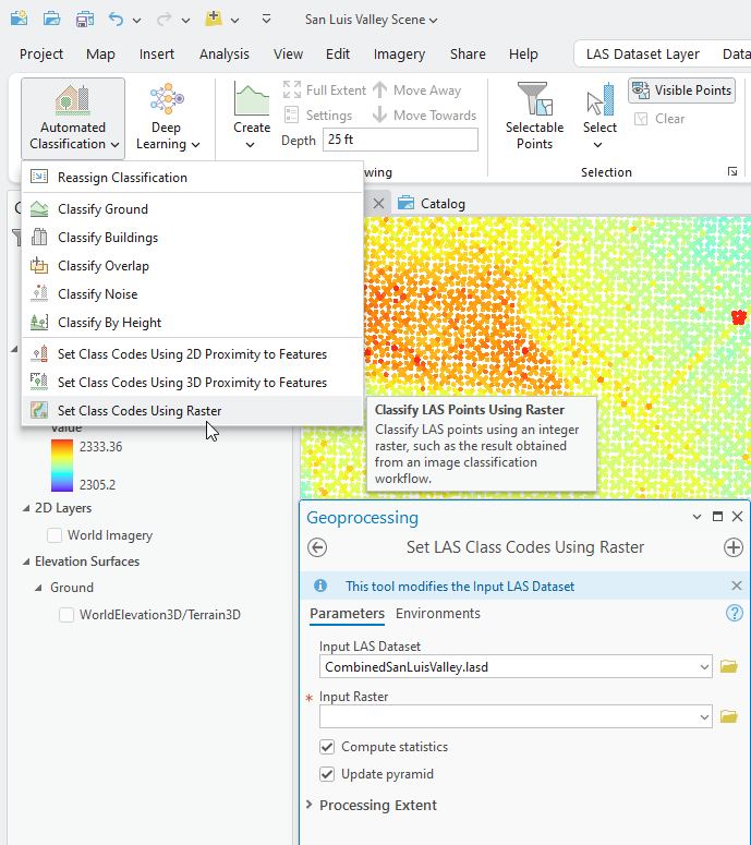
Under Automated Classification, eight tools are available—Classify Ground, Classify Buildings, Classify Overlap, Classify Noise, Classify by Height, Set Class Codes Using2D Proximity to Features,Set Class Codes Using3D Proximity to Features, and Set Class Codes Using Raster(Figure 20.3). This chapter will review some of the tools under Automated Classification, in the order shown. Note that whenever classifying points, ground points should always be classified first.
Let’s review each tool. Some will be demonstrated in the next chapter.
Select Reassign Classification, and the Change LAS Class Codes geoprocessing tool opens (Figure 20.4).
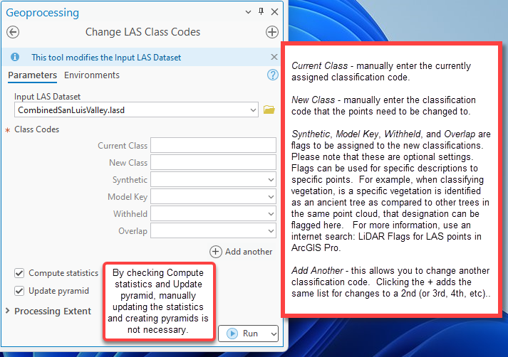
The Processing Extent, found here and in most other tools, is a very important decision to be made when using geoprocessing tools.
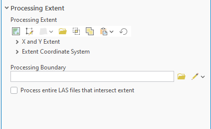
Expand Processing Extent. Processing Extent and Processing Boundary display (Figure 20.5). The change will apply to the entire dataset if Processing Extent is left as Default.
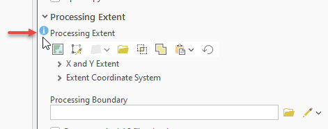
There are several options here to limit the processing extent (Figure 20.6). Point to the left of Processing Extent to activate the blue Information icon and select it.
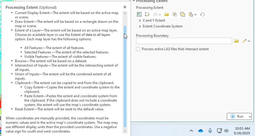
The information pop-up provides details on the Processing Extent options (Figure 20.7). For example, Current Display Extent will allow changes only to those points displayed in the map window. Extent of a Layer allows you to choose a layer within the map project to limit the scope of processing (listed in Contents). Browse allows the extent to be limited to that of another GIS file, for example, a vector feature class that defines a specific study area within the extent of the point cloud. Union of Inputs and Intersection of Inputs will be discussed with the Feature Proximity tools.
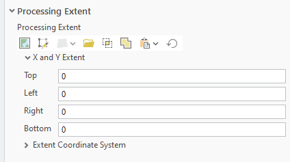
Expand X and Y Event. New input fields appear that allow entry of specific coordinates surrounding the points to be changed (Figure 20.8). Please note that not all points within these coordinates will be changed, only those from one type of classification code (current class that is entered as indicated in Figure 20.4) to another.
With the Processing Boundary (see bottom of Figure 20.6), a polygon can be created to encase the points to be changed. Clicking on the pencil icon lists Polygons as an option for the boundary. Selecting Polygons opens a drawing toolbar. This will be demonstrated in the next chapter.
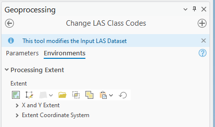
Select Environments. This tab provides another extent window (Figure 20.9).
Close the Change LAS Class Codes tool.
As mentioned previously, ground points should always be classified first. Go to Automated Classification and select Classify Ground. Some options are the same as the Reassign Classification tool—Processing Extent and Environments. These will not be reviewed again. Be sure to leave the Compute Statistics and Update pyramid boxes checked. Figure 20.10
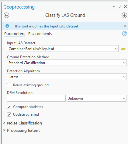
The additional decisions that need to be made to use this tool are as follows.
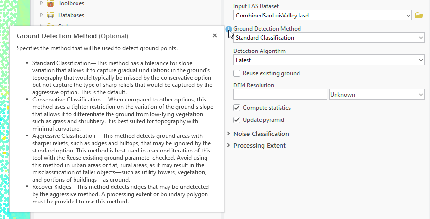
Ground Detection Method has three options—Standard Classification, Conservative Classification, Aggressive Classification, and Recover Ridges (Figure 20.11). Detailed information is provided about each of these methods; open the information icon for Ground Detection Method. The main difference in these methods is related to slope—a greater slope may affect how ground points are differentiated from low vegetation. Selecting the proper tool may be contingent on the topography of the study area.
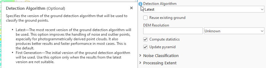
The next option for this tool is Detection Algorithm (Figure 20.12). This is an optional setting. Latest is the default, but you have the option to change this to First Generation. This option is utilized only when you have programmed a specific algorithm to use when classifying points (programming is beyond the scope of this book).
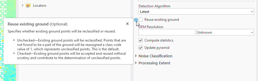
The next option for this tool is whether to reuse existing ground points (Figure 20.13). This option is typically selected when using the Aggressive Classification method in which existing ground points are not reclassified.
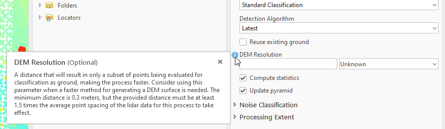
DEM Resolution is used if the classification of the point cloud is solely for the creation of a digital elevation model (DEM). The Unknown drop-down for DEM Resolution is for unit designation (feet, meters, etc.) (Figure 20.13). If classification of the point cloud will serve other purposes, such as identifying vegetation, do not use this option[1].
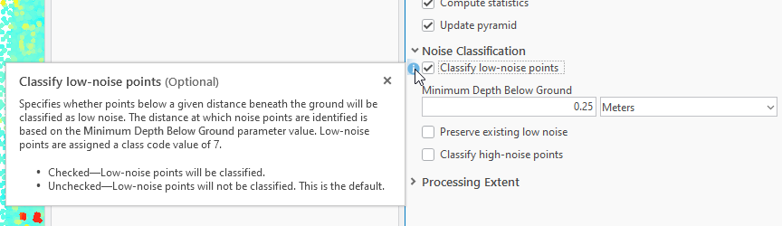
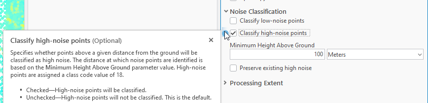
The next settings are under Noise Classification. Both of these settings are optional and are used to identify points that are considered “Noise”. Low Noise (Figure 20.15) identifies and classifies those points that are below ground level up to a specific depth below ground. High Noise (Figure 20.16) are those points above a specified height above ground level (an example of high noise would be an animal found within the scene on the date of acquisition). The noise options allow preservation of existing noise points and utilize both low and high noise settings at the same time. In both examples stated in the prior sentence, neither of those types of points (below ground or an animal) exist as a classification type in Table 1 at the beginning of this chapter.
Close the Classify LAS Ground tool and choose Classify Buildings. This opens the Classify LAS Building geoprocessing tool. Processing Extent, Environments, and Compute Statistics will not be reviewed—these have the same properties as other tools (Figure 20.17).
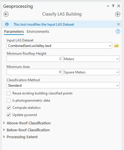
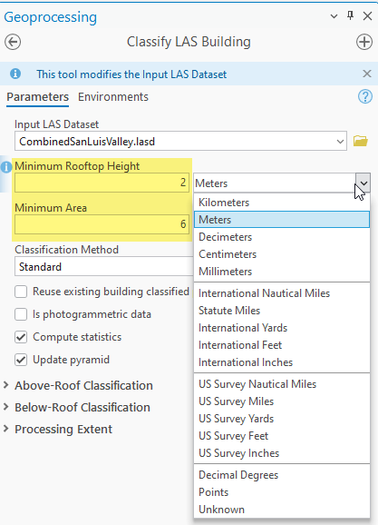
Within this tool, the Minimum Rooftop Height and Minimum Area are designated. Use the default values (2 and 6, respectively) or enter specific values. Using specific values can be very useful in an urban area with large and tall buildings. Be careful in residential areas, as trees can be misinterpreted as buildings. The unit of measurement can also be changed (meters or feet, for example). Figure 20.18
If Reuse existing building classified points is not checked (Figure 20.18) and building classified points are already present, those points could be reclassified as unassigned if they don’t meet the parameters established under Minimum Rooftop Height and Minimum Area. If some points are correctly classified as buildings, it is recommended that this box be checked so those points are not reassigned and could assist in identifying other building points (Figure 20.16).
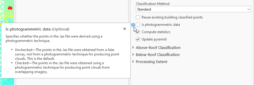
The next option is Is photogrammetric data (Figure 20.19). This box is only checked if the point cloud was derived from a photogrammetric technique. If the point cloud was a lidar acquisition, this box is not checked (thus unchecked is the default).
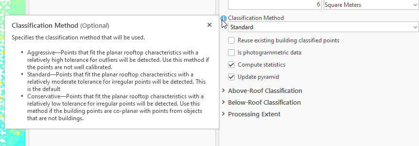
Now we look at the Classification Method (Figure 20.20). This is very similar to the classification methods under Classify Ground (considering slope), and for Classify Building related to rooftops characteristics. Which method to use will likely be highly dependent on rural (similar rooftop characteristics) vs urban (varies from small homes to high rise buildings) environments.
Close the Classify LAS Building tool and open Classify Overlap (Figure 20.21). The Classify LAS Overlap tool is only used for overlapping scans with differing scan angles. Lidar data with larger scan angles may cause some irregular point distributions and larger than desirable margins of error. This can occur if the lidar tiles added to a LAS dataset do not come from the same acquisition or if problems develop during the flyover[2].
Close Classify Overlap and open Classify Noise (Figure 20.22).
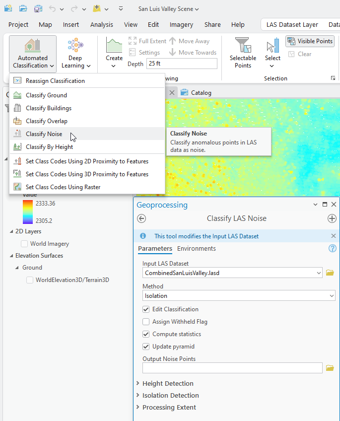
Noise was introduced in Chapter 15. Lidar Display Settings, but as the Classify LAS Noise tool in Figure 20.22 shows, noise are points with anomalous spatial characteristics in the dataset. Points classified as noise are not used in most analyses, so many decisions must be made when identifying points as noise.
The processing extent is the same as that of other tools already discussed.
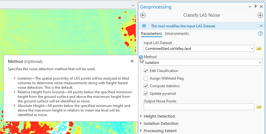
There are three options for the Method of noise identification—Isolation (the default), Relative Height from Ground, and Absolute Height. Each description is visible in Figure 20.23.
Recall from Table 1. Classification Codes for Lidar Returns that there are two classification codes for noise—7 Low Noise and 18 High Noise. In many instances, the raw data provided to the customer already has some noise points identified (the reason noise class codes are already present in this San Luis Valley dataset).
Which of these methods is appropriate?
Isolation, the default (Figure 20.23), allows ArcGIS Pro® to evaluate the dataset looking for the anomalies. Some parameters for this method can be changed.
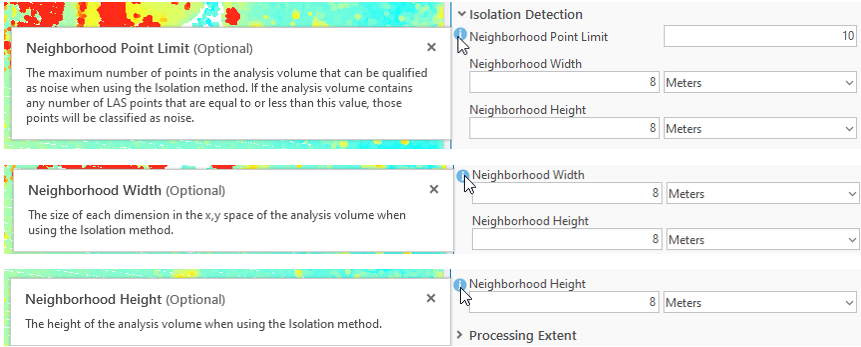
Expand Isolation Detection (Figure 20.24).
The Neighborhood Point Limit is already set at 10. This limit is the maximum number of points within the designated area (neighborhood, defined by the width and height settings) that can be classified as noise. If the dataset has a much larger number of points within the neighborhood that qualify as noise, the validity of the dataset should be questioned. The Neighborhood Width and Neighborhood Height are already set at 8 meters; these values can be increased or decreased, and the unit of measurement changed.
The settings that should be used will be dependent on knowledge of the area.
Under Height Detection (Figure 20.25), the minimum and maximum heights for ground values are set. Those values may be difficult to determine if the area has substantial relief, so if a raster file is available for the ground and it has an elevation value in the attribute table, it can be added under Ground Raster Surface. If the area of interest is flat, such as an agricultural field of soybeans in Iowa, the minimum and maximum heights could easily be established without a ground elevation raster file. You will need to identify the unit of measure as the default setting is unknown.
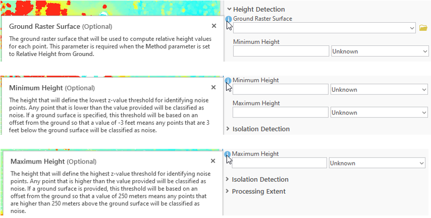
Suppose the exact elevations of the region are not known, but it is known that certain values above and below ground should definitely be noise (for example, 10 meters below and 100 meters above), use the Relative Height from Ground method. In that case, the Minimum Height and Maximum Height values are entered here under Height Detection.
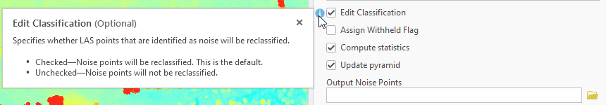
As with other classification tools, already classified points can be included when using this tool. Unlike other tools, which do not include them as the default, this tool includes them by default because the analyst is establishing the specific parameters for noise (Figure 20.26).
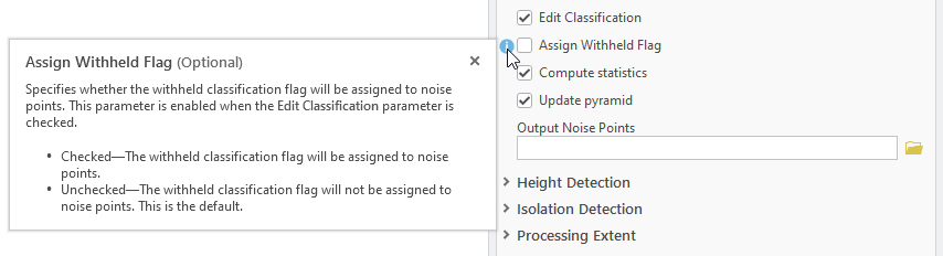
Assign Withheld Flag is unchecked by default (Figure 20.27), which means the points are not withheld from any other dataset processing, so the points are still available if they are needed in other processing or if they are then identified as something other than noise. An example of this would be a low point, which has an evaluation value of 100 meters below the lowest nearby ground point. A field evaluation of the area later determines that this was the first sign of a sinkhole. Thus, further assessment of the initial lidar point cloud may be necessary, and low noise points included.
Output Noise Points is an optional setting (Figure 20.28). Use this if a new feature class of just the noise points is desired in addition to the classification.

Which method or which optional setting should be used with these tools depends on familiarity with the region. The more familiar an analyst is with the region, the more optional parameters can be included, or default values be changed.
Close Classify Noise and open Classify by Height. The Classify LAS By Height tool allows classification of multiple classification codes at one time (Figure 20.29). This tool will be demonstrated in the next chapter.
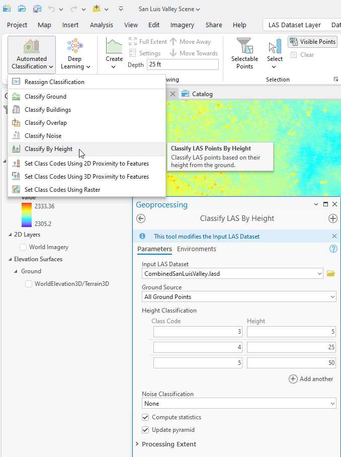
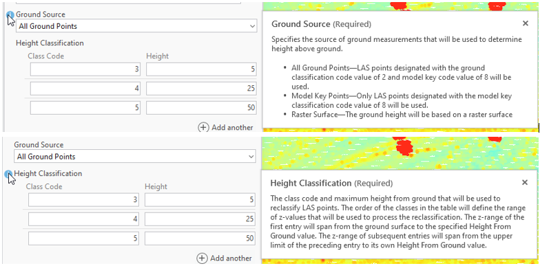
A Ground Source is required because the height values reflect height above ground.
The points classified as Ground in this dataset can be used in this specific setting, so ground points should always be classified first. The default Class Code values already present in this tool are vegetation codes. These can be changed, for example, when classifying buildings in urban areas or classifying areas with little vegetation and mainly manmade structures. The Height values can also be changed—another reason familiarity with the study area is necessary. Does low vegetation include soybeans, medium vegetation corn, while high vegetation refers to oak trees? Or does low vegetation mean bushes, medium vegetation mean oak trees, and high vegetation mean redwoods?
Please note that this tool only classifies unassigned points. Any points already assigned should not be changed (Figure 20.30).
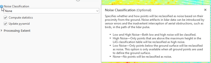
The last option to discuss in this tool is Noise Classification (Figure 20.31). Compute Statistics, Update pyramid and Processing Extent work the same as in other tools already discussed.
Be careful when changing the Noise Classification option. Changing from the default (None) will classify all unassigned points outside of the Height Classification parameters as noise.
Close Classify by Height. The next three tools use feature classes or a raster dataset to assist in classification of points. Open Set Class Codes Using 2D Proximity to Features (Figure 20.32).
The Input Feature Class (a required input) does not have to be in the project but can be stored on the computer. For example, if a buildings shapefile (or feature class) exists, it can be used to help classify the points that are 6 Building. This tool can also assign Flags to classified points. See Figure 20.33.
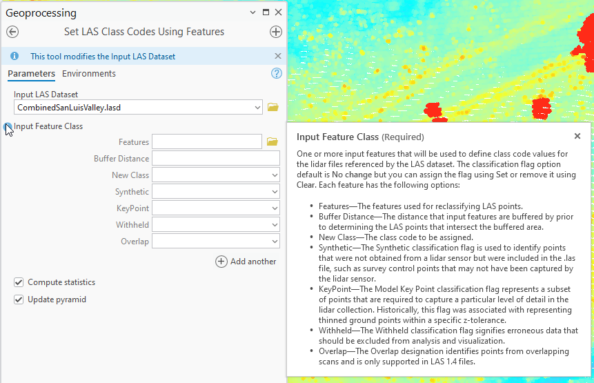
You can use the + sign to Add another feature class to be used in assisting the classification (Figure 20.33). Perhaps there is a point feature class for city park trees in addition to a building shapefile. Using Buffer Distance can help identify those points in a point cloud that are tree canopy (a buffer distance around the point).
For this tool, the Processing Extent is found only in Environments but all the settings are the same as the other tools (Figure 20.34).
Close 2D Proximity and open Feature Proximity > 3D Proximity (Figure 20.35).
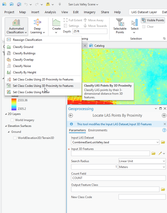
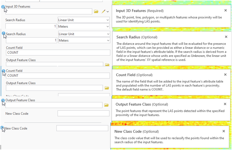
This tool is much more complicated than the 2D tool. It requires a 3D feature class. Instead of a buffer distance, it uses a Search Radius (remember this is x, y, and z). This tool will add a new field to the 3D feature class, named Count, or a different name can be designated. An optional Output Feature Class can be created for those classified points, and a field to add the New Class Code assigned to those points. (Figure 20.36.)
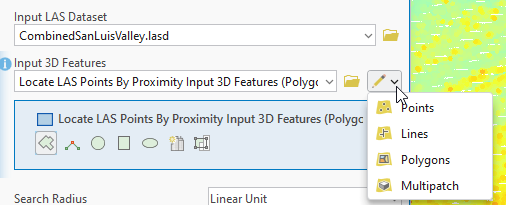
If no 3D feature class exists, this tool allows for creation of one (Figure 20.37). Click on the pencil icon at the end of the Input 3D Features line, and a list of possible file types will appear. Choose the appropriate feature (point, line, polygon, or multi-patch). In Figure 20.37, Polygons was chosen. The create polygon tool opens, as happened during the discussion of the Reassign Classification tool. Thus, a new 3D feature class is created, which is then used to classify points.
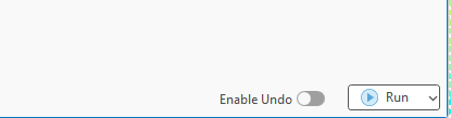
At the bottom of the geoprocessing window is an option not seen in any other tool—Enable Undo (Figure 20.38). This is the only tool which allows the geoprocessing operation to be undone. The default setting is off. Selecting the button turns it on.
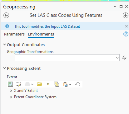
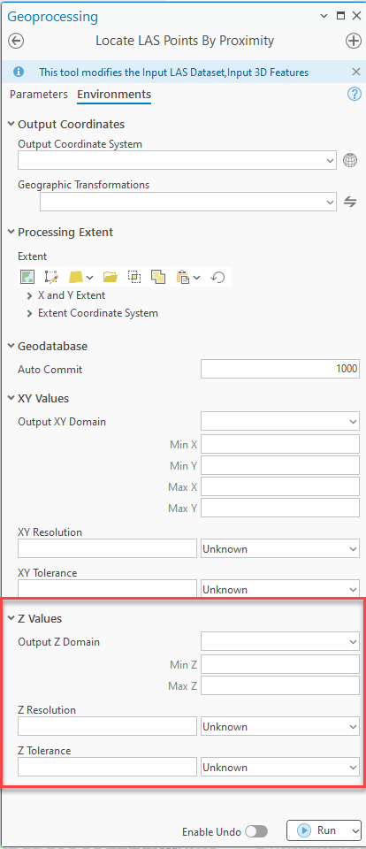
The last settings to discuss in this tool are under Environments (Figure 20.39). This includes Output Coordinate System (if creating an output feature class), Geographic Transformations (remember possible coordinate system differences), and entering the Processing Extent for processing. The Processing Extent options are the same options as in previous tools, but this is 3D, so the coordinates for As Specified Below also include Z values.
The final tool to discuss is Set Class Codes Using Raster (Figure 20.40). This tool uses an existing raster dataset to assist in the classification of points. We will discuss the tool briefly here but will not demonstrate the tool in the next chapter.
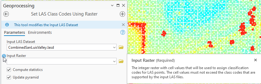
The Compute statistics, Update pyramid, and Processing Extent settings are the same as with other tools. The Input Raster entry (Figure 20.41) utilizes a raster data set with a cell value that is integer based (whole numbers) and these numbers must correspond to the LAS classifications codes (Table 1 at the beginning of this chapter).
This concludes the introduction to geoprocessing tools for classifying points in a point cloud. The next chapter will demonstrate the Classify by Height tool, the Reassign Classification tool and the Set Class Codes Using 3D Proximity to Feature tool.
