Chapter 19. Interactive Classification
The prior chapter introduced classification codes. This chapter will demonstrate how to classify individual points (or groups of points) interactively. Table 1 provides a reminder of the classification codes discussed in the previous chapter.
| Classification Value | Classification Description |
|---|---|
|
0 |
Never classified |
|
1 |
Unassigned |
|
2 |
Ground |
|
3 |
Low Vegetation |
| 4 | Medium Vegetation |
| 5 | High Vegetation |
| 6 | Building |
| 7 | Low Noise |
| 8 | Reserved |
| 9 | Water |
| 10 | Rail |
| 11 | Road Surface |
| 12 | Reserved |
| 13 | Wire – Guard (Shield) |
| 14 | Wire – Conductor (Phase) |
| 15 | Transmission Tower |
| 16 | Wire-Structure Connector (Insulator) |
| 17 | Bridge Deck |
| 18 | High Noise |
| 19-63 | Reserved |
| 64-255 | User Definable |
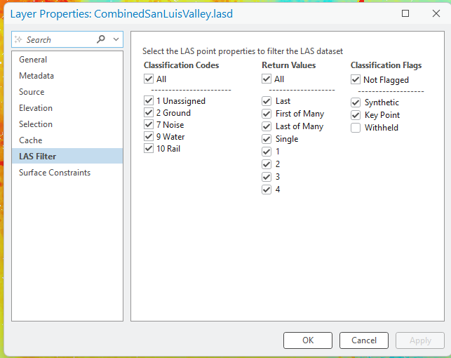
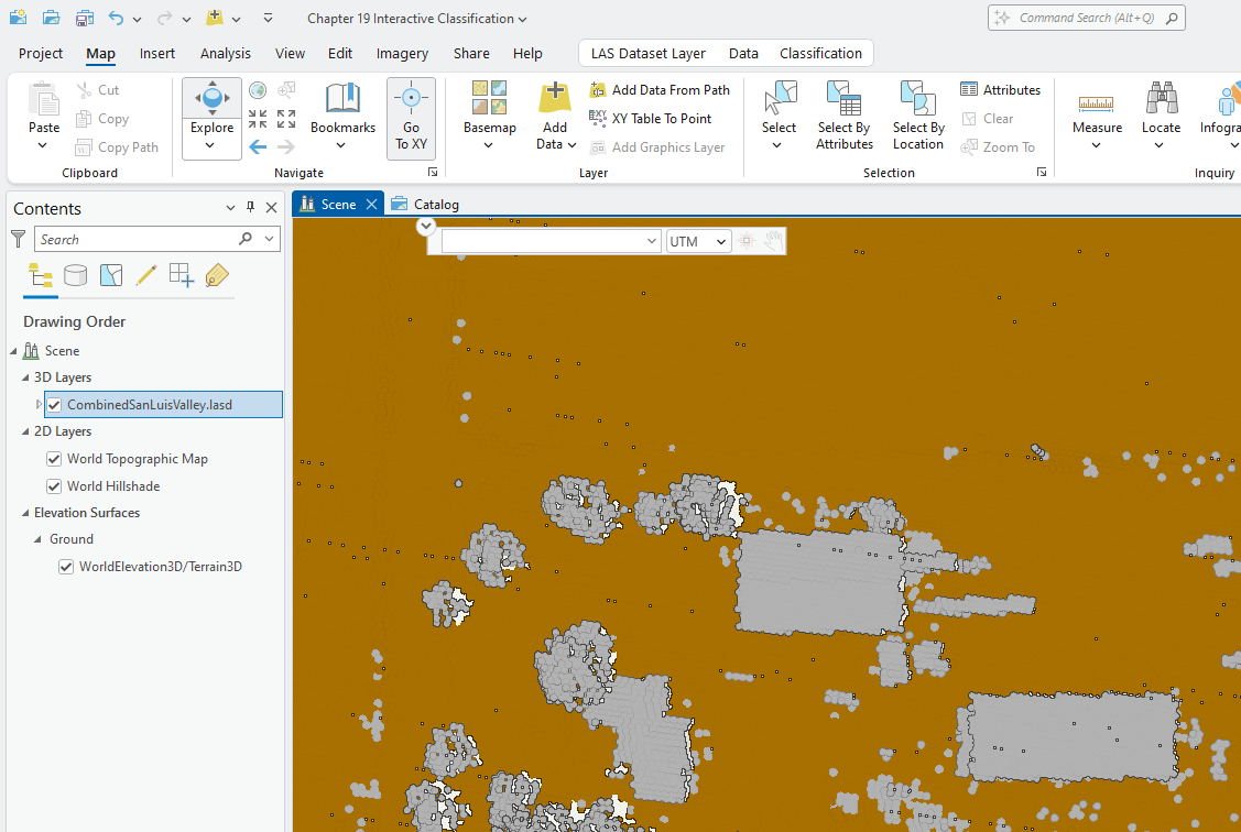
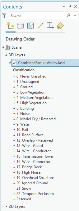
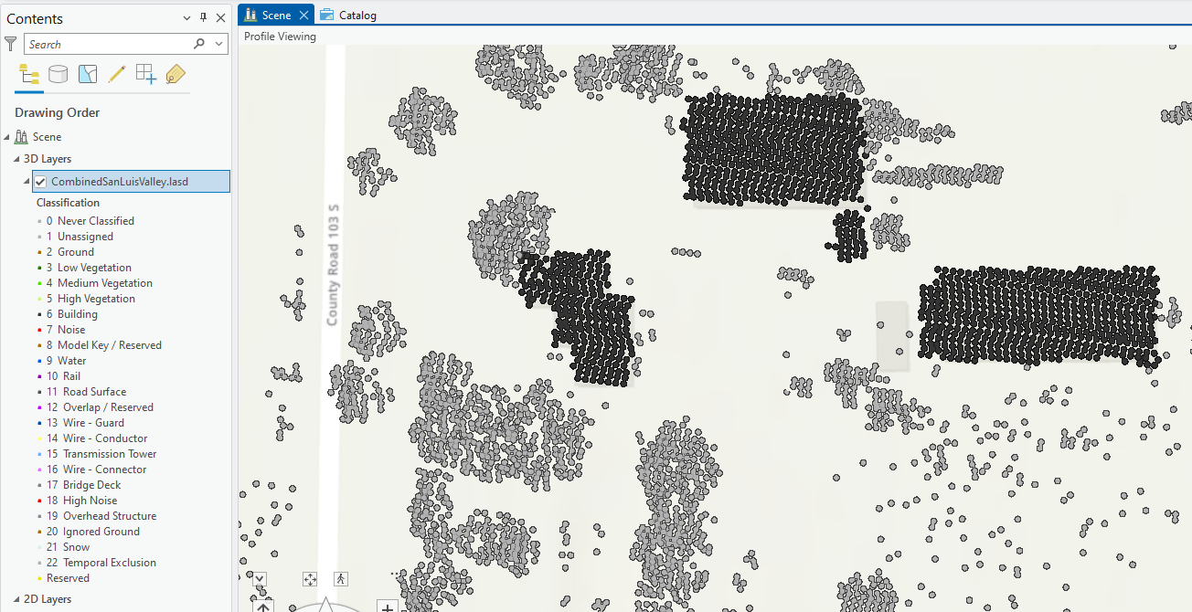
Open a new map scene and add the San Luis Valley .lasd dataset. Open Properties and go to LAS Filter. Five (5) Classifications already exist—Unassigned, Ground, Noise, Water and Rail (Figure 19.1). Noise are those points that appear to be below ground level.
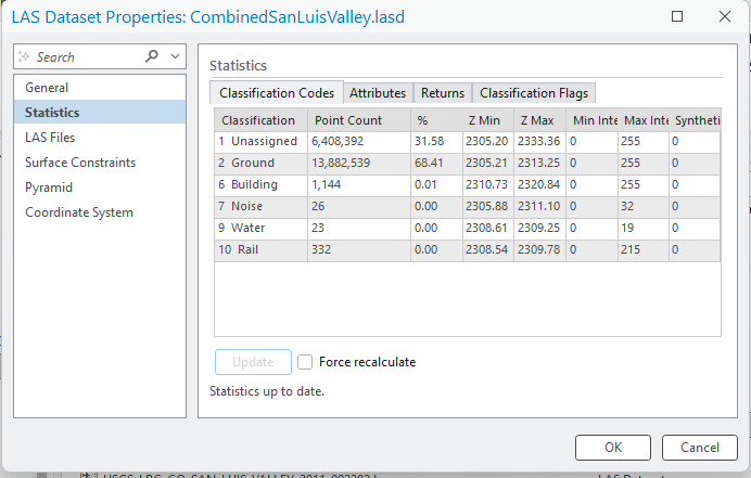
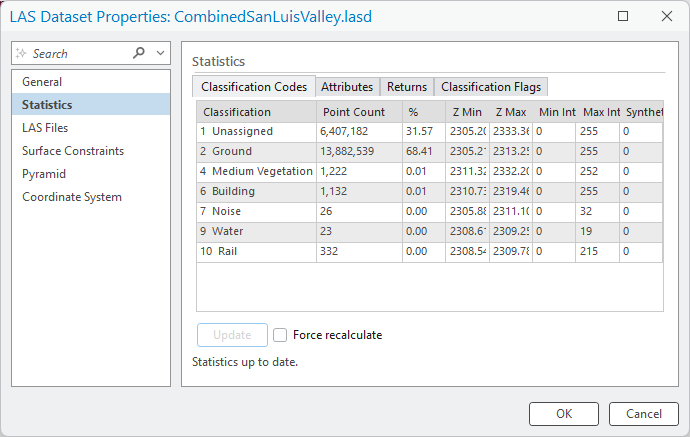
From a Catalog View of the LAS dataset, determine how many points are assigned to each classification (Figure 19.2).
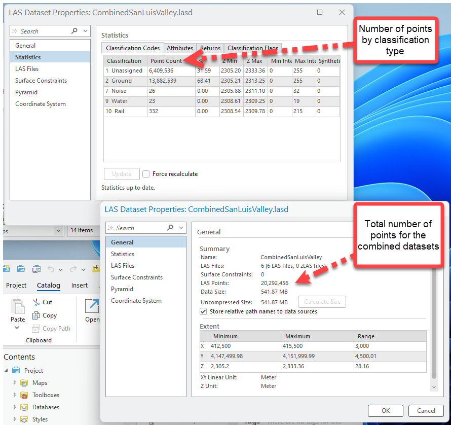
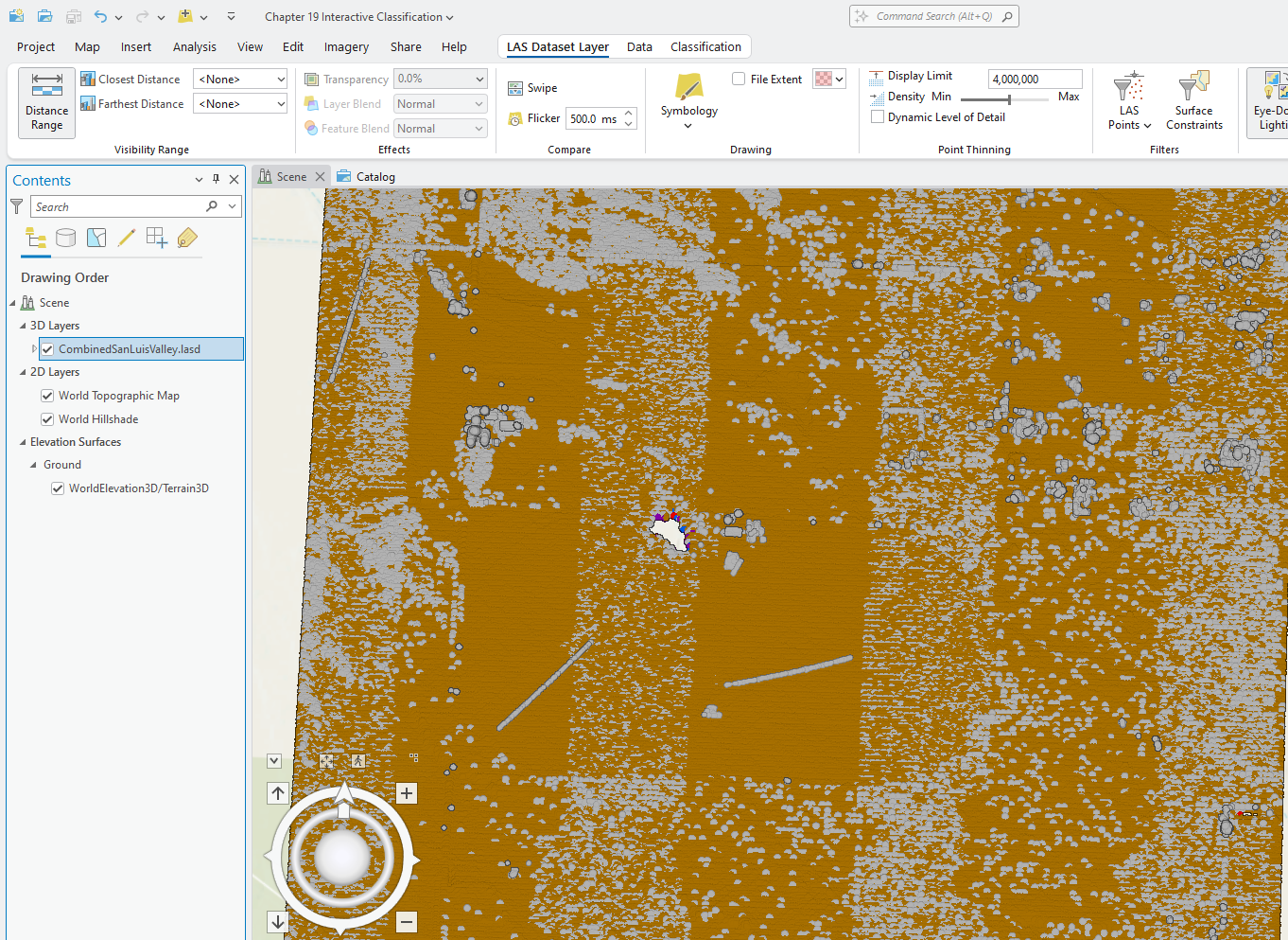
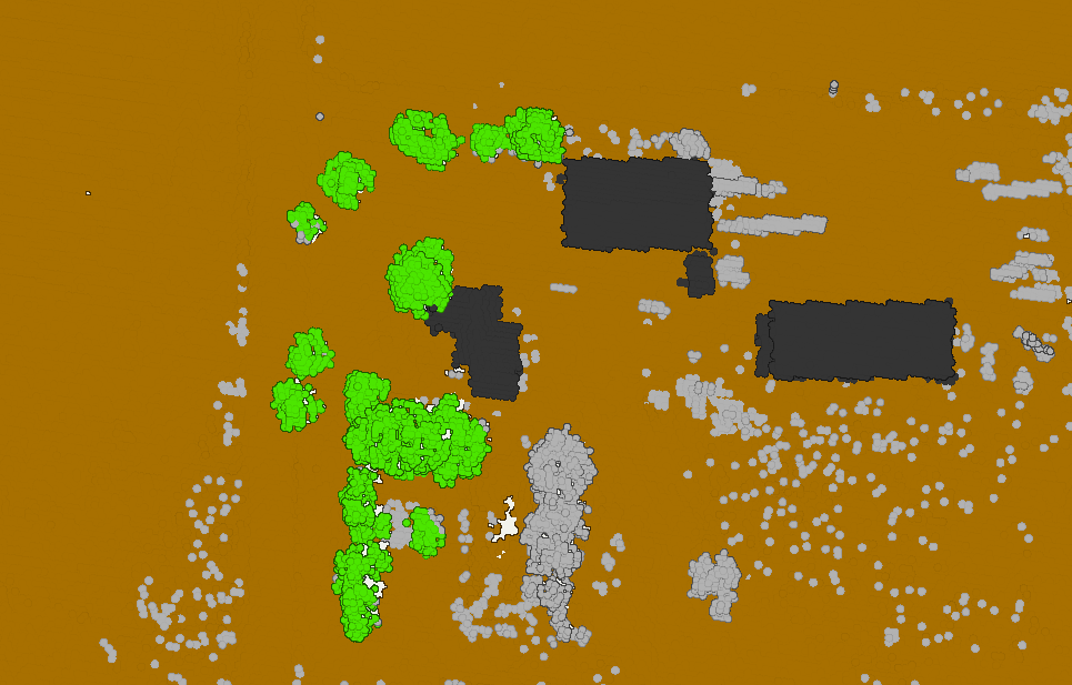
Of the 20,292,456 points in the point cloud, 6,409,536 (almost 32%) are not classified (unassigned). Navigate through the point cloud. Notice that buildings, vegetation, roads, electrical wires (among other features) are present but are not assigned to any classification code. Change the Symbology to show classification codes and change the colors so that each class is easily distinguishable (Figure 19.3).
Zoom in to the area shown in Figure 19.4.
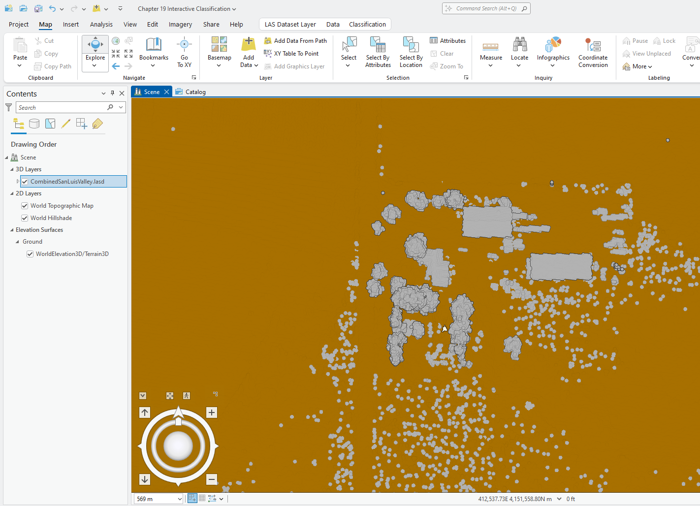
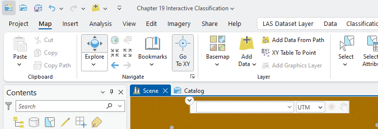
Are you having difficulty finding the location? Use Go to XY in the Map tab (Figure 19.5) and use the coordinate values on the status bar (413,019E; 4,150,454N) in Figure 19.4 to navigate to the correct region of the map display.
Now, zoom in to the two buildings in the north (Figure 19.6).
Note: When classifying points, the original dataset is being changed. Unassigned points will be assigned a classification here.
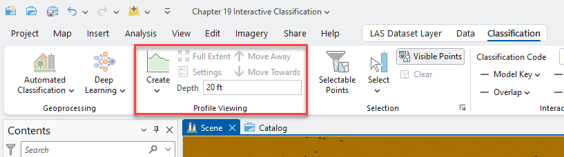
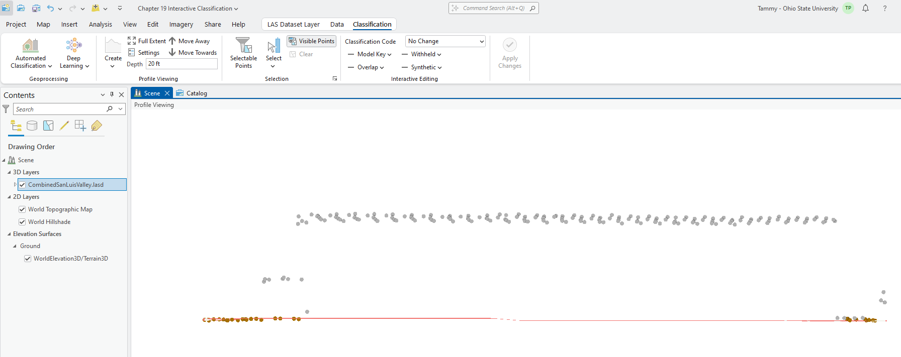
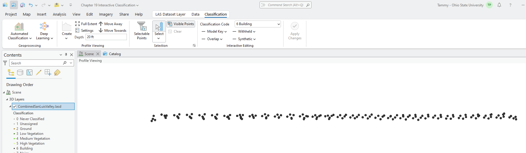
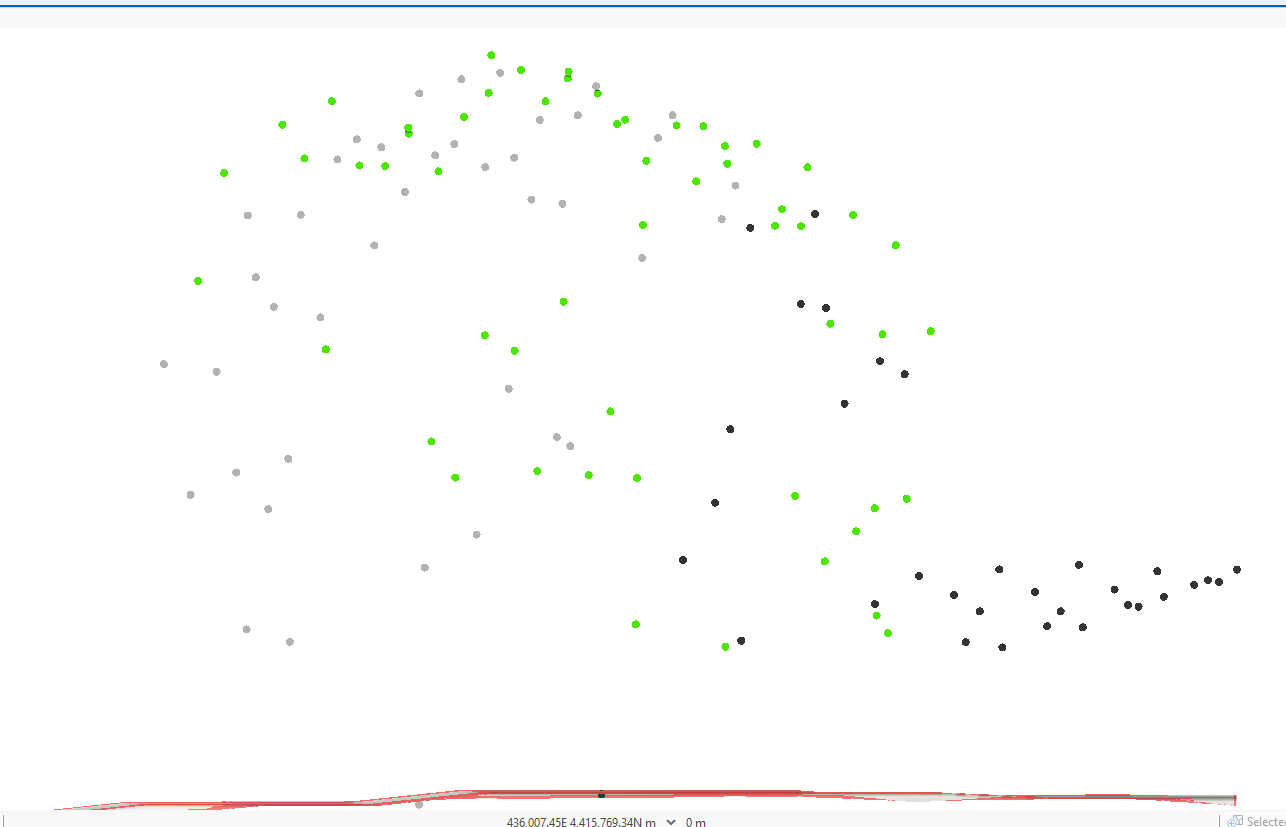
Remember how do to Profile View? Click on the Classification tab. Create profile will be used to create a vertical slice to assist in classifying (Figure 19.7).
Create a Profile View on the building as shown in Figure 19.8. Make the depth 20 feet and be careful to include only roof/building points.
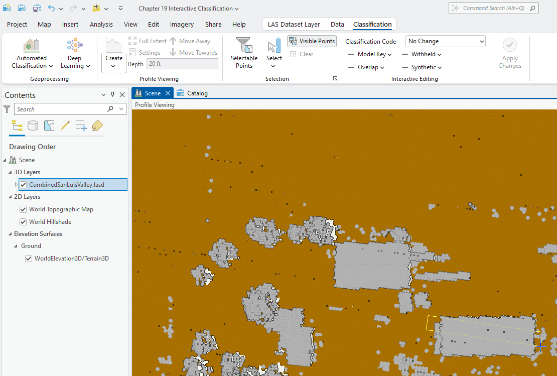
Zoom out in the Profile Viewing window, so all points are clearly seen within the window (the only points from the point cloud that are seen in Profile Viewing are those within the box created). Figure 19.9. Don’t close Profile View!
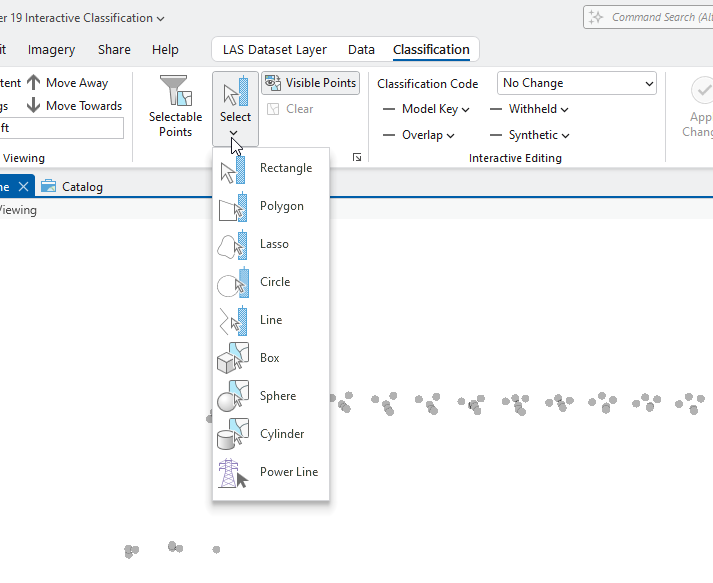
Click Select from the Selection Group in the Classification tab. You will be using this to select specific points to classify. You can select these using a variety of shapes.
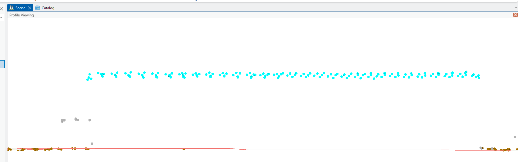
In the Profile Viewing window, drag a rectangle around the roof/building points to select them (Figure 19.11). Take care to capture only roof/building points.
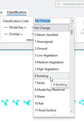
In the Interactive Edit Group, click the drop-down arrow for Classification Code (initially contains No Change) to find the list of classification codes available. (Figure 19.11).
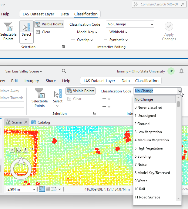
Choose the code 6 Building (Figure 19.13).
Ensure 6 Building appears in the Classification Code box and click Apply Changes (Figure 19.14).
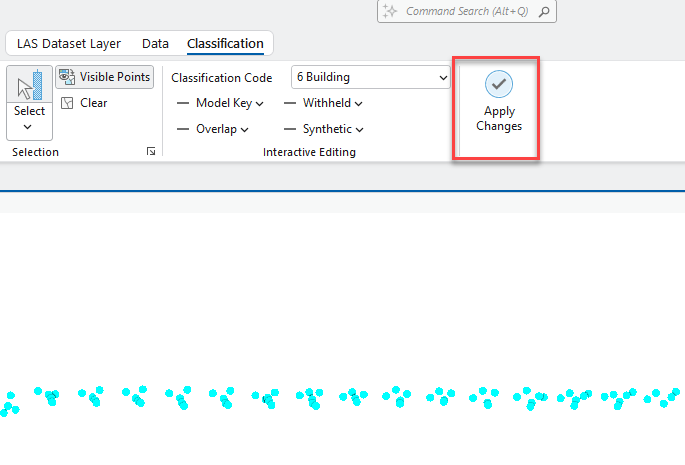
It initially appears that the points have disappeared (Figure 19.15), but once it reloads the points will be colored in the new classification.
Close the Profile Viewing window. Not all of the roof was classified as building. Interactive classification only classifies the points within the selection frame. (Figure 19.16).
In Contents, all classification codes available within the San Luis Valley dataset are now displayed, even though not all classification codes are used in this point cloud. The building points are now showing (Figure 19.17). Recall from the prior chapter, although there can be up to 255 different codes (64 – 255 user-defined), the classification codes available within a dataset are determined by the dataset owner. So, for the San Luis Valley dataset, these are the only classification codes that can be used. If your classification symbology did not update, go to the symbology tab and redo the symbology.
Using Select within Profile Viewing was only one way to interactively classify points.
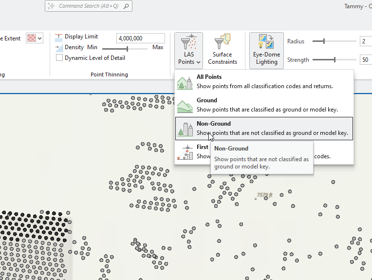
Zoom in closer to the same building. The Select tool can also be used outside of Profile Viewing. But, first change the LAS Points display to non-ground (Figure 19.18).
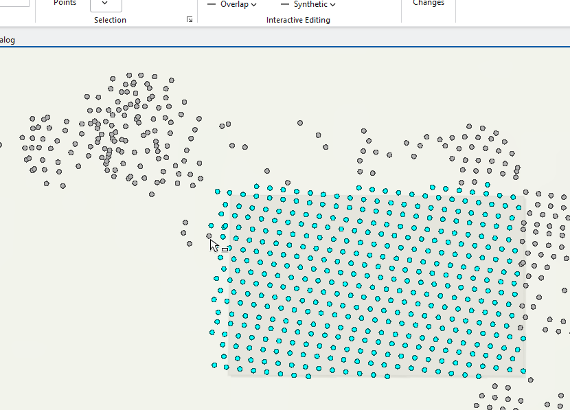
Next, drop-down Select and try doing the selection as shown in Figure 19.19, using Rectangle (or a shape with which you are comfortable). If necessary, for example if ground points are included, use Clear to start over.
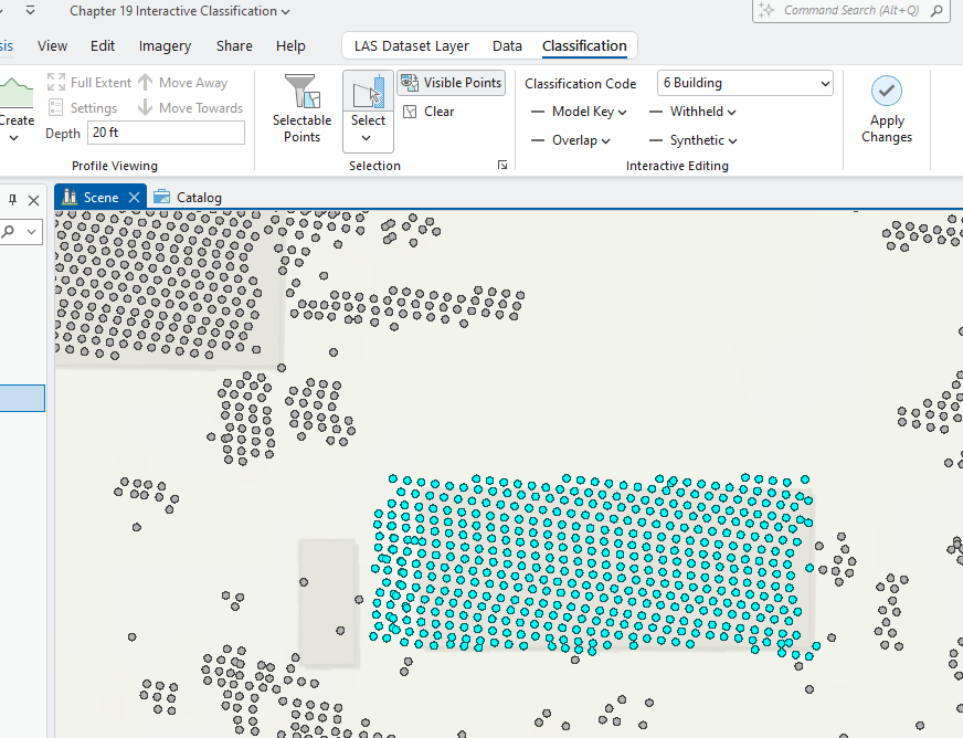
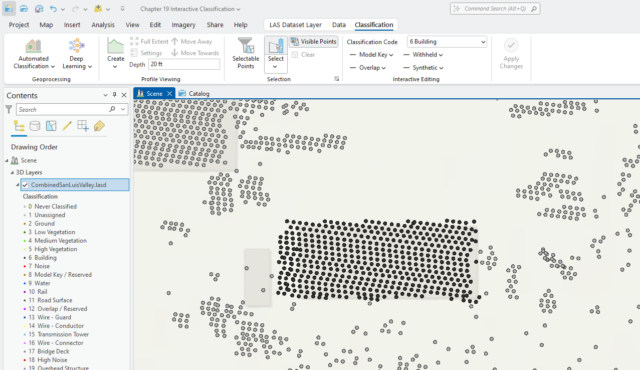
Make sure Classification Code is 6 Building, then click Apply Changes. Sometimes, it takes a few seconds to apply the changes and reload the points (Figure 19.20). There is no need to update the Symbology.
But now go to Catalog View to check Properties > Statistics to be sure this new Classification Code has been added to the dataset’s statistics. It has not, but does have the message 1 file(s) have outdated or no statistics. (Figure 19.21).
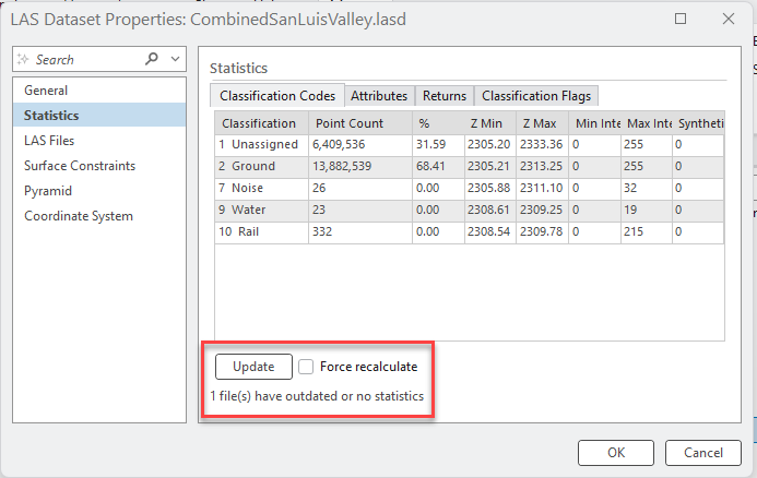
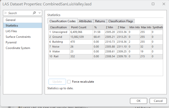
As the interactive classification process is completed, Statistics must be updated. Remember how to recalculate? Click Update (red box in Figure 19.21). Statistics are now updated and 6 Building classification is now showing (Figure 19.22).
Go back to the Scene. Continue classifying the building points. Practice with the different selection methods—Polygon, Lasso, Circle and Line (as seen in Figure 19.10).
Note: When using interactive selection, if a point is missed in the process, hold down shift and click individual stray points to add them to the selection (Figure 19.23).
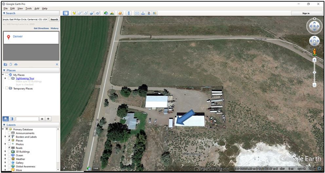
Use reference images to assist in classification if necessary. For example, there are unassigned points shown at the left of the roof in Figure 19.23. Are these building or bushes next to a building? Figure 19.24 is the same region displayed in Google Earth® and makes clear that those additional unassigned points are roof/building.
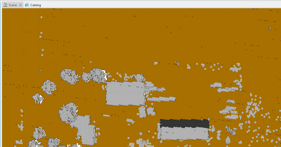
Continue with this classification process until all buildings in this extent are classified as 6 Building (Figure 19.25). Remember to Apply Changes to save the work.
Don’t forget to update Statistics (Figure 19.26)! If the point count under 6 Building is a few off from Figure 19.26, don’t worry, those will be addressed in Chapter 21.
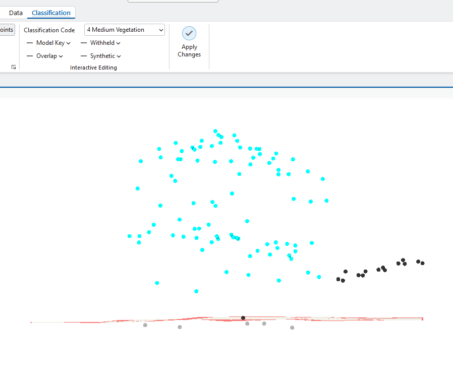
For additional practice, do a few of the trees in this extent. Use 4 Medium Vegetation, not 5 High Vegetation. Why trees in 4 Medium Vegetation? Trees vary in height—trees such as sequoias and redwoods in California will be much taller and, thus, qualify as 5 High Vegetation.
Trees are best completed in Profile View so no understory vegetation such as perennial flowers and bushes are captured. (Figure 19.27) And Apply Changes in Figure 19.28.
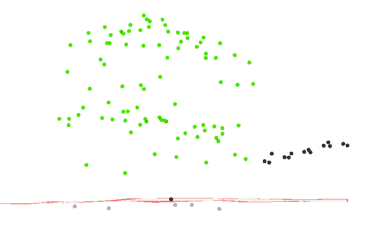
It may be necessary to create a Profile View from different perspectives to capture all of the points (Figure 19.29).
When finished, it may look like some points were missed (Figure 1930), but trees allow lidar pulses through and some of these may be ground or understory vegetation. These will be addressed in Chapter 21. Classifying Points Using Geoprocessing Tools.
When finished, don’t forget to update Statistics again (Figure 19.31)!
Yes, this is a long, monotonous way of classifying points. This method is best used when classifying points in a
very small area, a large area where all points are the same (so a large number can be selected at the same time), or when classifying a small number of incorrectly assigned points.
Additional classification methods are available and will be covered in the next two chapters.
