Chapter 17. Using Profile View

A Profile view provides a 2D vertical view of a specific region in the point cloud, unlike navigating through a 3D scene. Profile view provides information about the area of interest. It is an essential tool in classifying unassigned points.

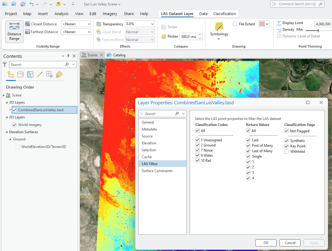
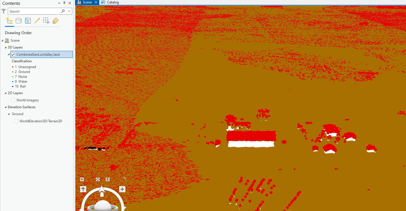
Create a new local scene and add the San Luis Valley .lasd file. Open Properties and go to LAS Filter. Recall that five classifications exist—Unassigned, Ground, Noise, Water, and Rail (Figure 17.1).  Note: Noise could explain the points that appear to be below ground level. Classification schemes will be discussed in more detail in the next chapter.

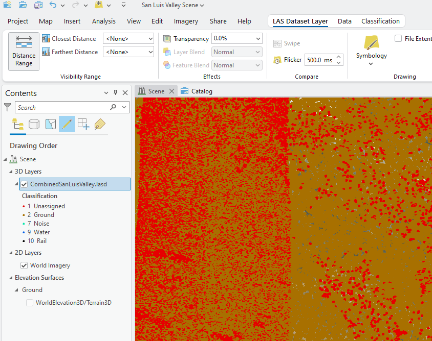
Change the symbology to show the classification codes and change the colors so that each class is easily distinguishable from the others (Figure 17.2).

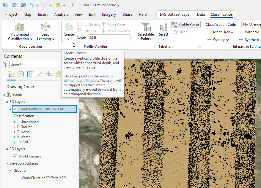
Click on the Classification tab (Figure 17.3). Create profile in the Profile Viewing group will be used to view the classified points with a vertical slice (Figure 17.3).

Follow along step-by-step. Ensure Auto-complete is checked by clicking the down arrow under Create (Figure 17.4).

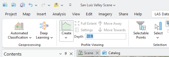
Profile Viewing includes the depth of the profile (20 ft, highlighted in blue in Figure 17.5). This depth can be changed, increased, or decreased. The depth used depends on the area being viewed. If it is bare ground, the depth can be increased as it is unlikely that the points would be related to anything but ground. However, in forests and urban areas, for example, features can vary greatly even within 10 feet, so the depth may need to be decreased. Leave as default here.

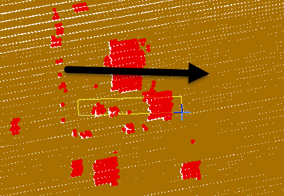
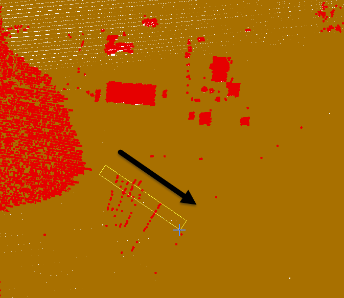
Now, select Create and click once in the scene (Figure 17.6). Move the mouse in the direction of the black arrow (note that the arrow was placed on the figure below for illustration; it is not present in ArcGIS Pro®), and once the yellow line extends as shown, click again (Figure 17.6) to complete drawing the profile line.

The profile window opens (Figure 17.7).

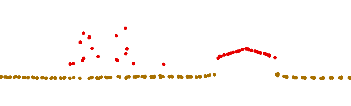
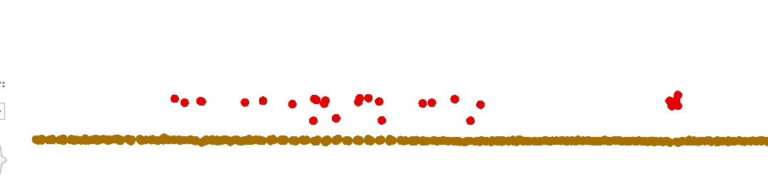
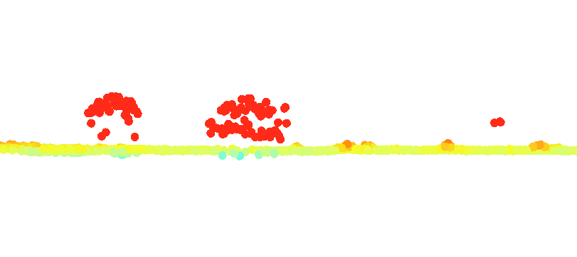
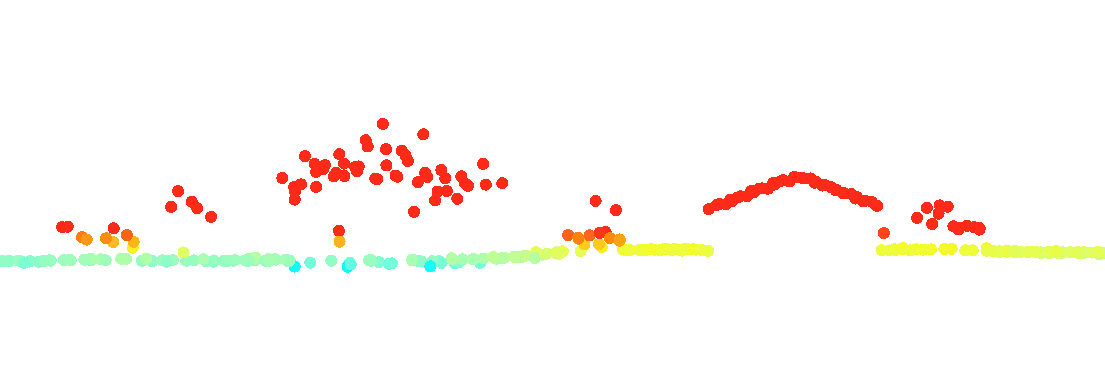
Use the mouse wheel to zoom in and out. Zoom in to the area between the cluster of red points on the left and red points on the right (Figure 17.8). From the symbology, red points are unassigned points. What feature is represented by the row with the peak? What about the cluster of unassigned points on the left? Notice some unassigned points are also intermingled with ground points (brown).

Exit Profile Viewing by clicking the close button—the red box containing an X in the upper right corner of the Profile Viewing window.

Now zoom in to the area where the Profile View was initiated (Figure 17.9). The straight row of unassigned points are roof lines for buildings, and the clusters are likely trees.

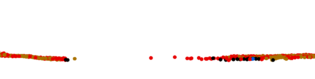
Leaving the extent in the map window as shown, put the viewer back to overhead view, change the depth to 30 feet and do another Profile View as indicated by the black arrow in Figure 17.10.

From the results shown in Figure 17.11, it appears that the unassigned points are higher than ground.  Are these also ground because the ground is not actually level or are they very low vegetation? This is just one decision that must be made when classifying points. Familiarity with the area of interest is essential.

Practice using Profile View, changing the depth settings, changing the length of the box, and moving around the scene.

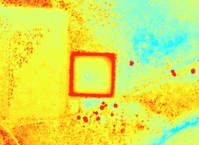
Try to locate the area in Figure 17.12. What type of feature could cause a break in the point cloud? (A water body because clear, deep, calm water absorbs the points and results in no returns).

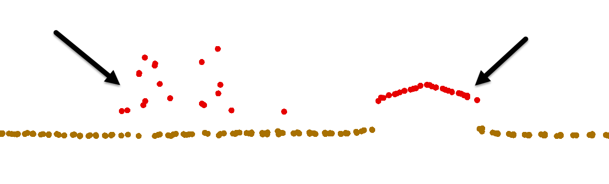
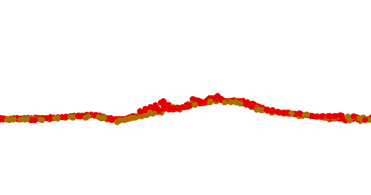
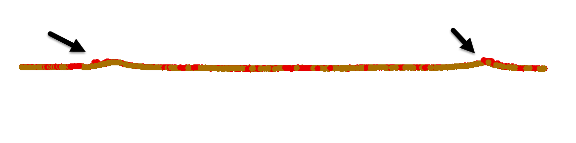
What about the feature in Figure 17.13? The top image is one side of the feature.

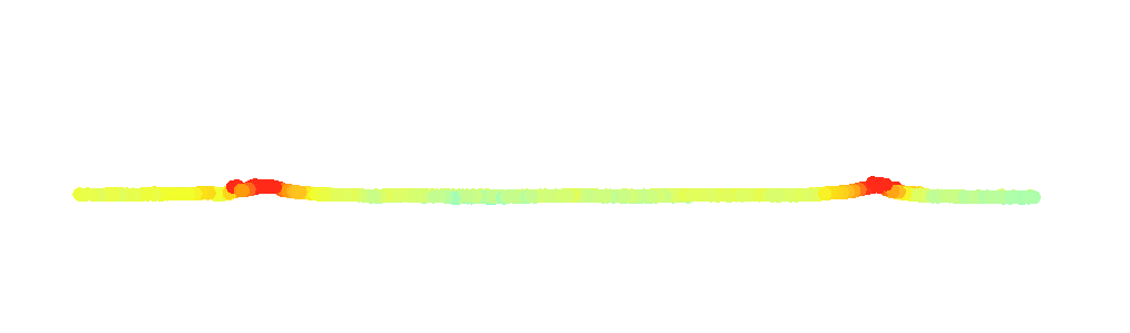
Figure 17.14 is a profile view that includes both sides of the feature (the black arrows are pointing to the slight rise on each side).  A hint is in Figure 17.15 using elevation symbology.

Change the Symbology to elevation and redo the same Profile View in the center image in Figure 17.14 (result in Figure 17.14).

Practice using the Profile View of the trees just south of that feature (Figure 17.17).

Practice using the Profile View of the trees and buildings to the east (Figure 17.18).

Sometimes, changing the symbology does not help with feature identification; sometimes, it makes a big difference. The symbology, along with other tools discussed in prior chapters, will greatly assist when classifying points. Profile View will also be very helpful when classifying unassigned points.

The next four chapters introduce classification schemes and the discussion of classifying unassigned points.