Chapter 15. Lidar Display Settings

The last two chapters introduced adding lidar data as separate tiles and then combining separate tiles to generate a single LAS(.lasd) dataset. As noted in those chapters, ArcGIS Pro® does not display the entire point cloud and, in some instances, does not display any part of the point cloud until zoomed in to a portion of a tile. This chapter introduces the settings that control the display and demonstrates how to display only certain classification codes and/or returns.

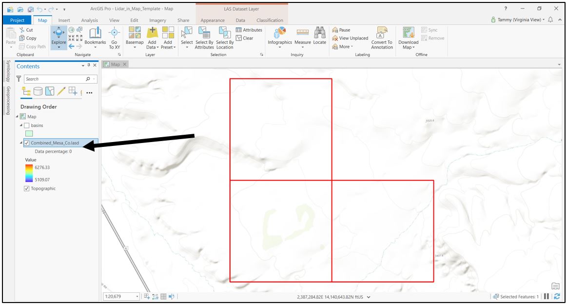
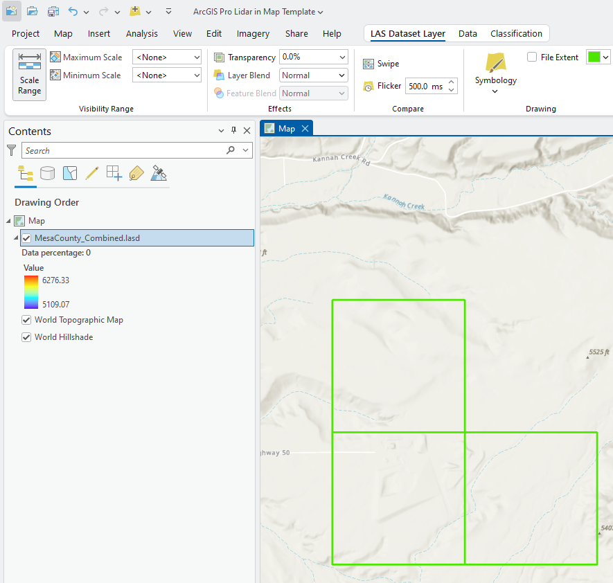
Start with the Mesa County Colorado data, the map created in Chapter 10. Setting up ArcGIS Pro for Lidar Data. Recall that, at full extent, just the footprint of the data displays, not the actual data (Figure 15.1). Under the layer name in the Contents tab note the indication: Data percentage 0. This means that none of the point cloud data are displayed.

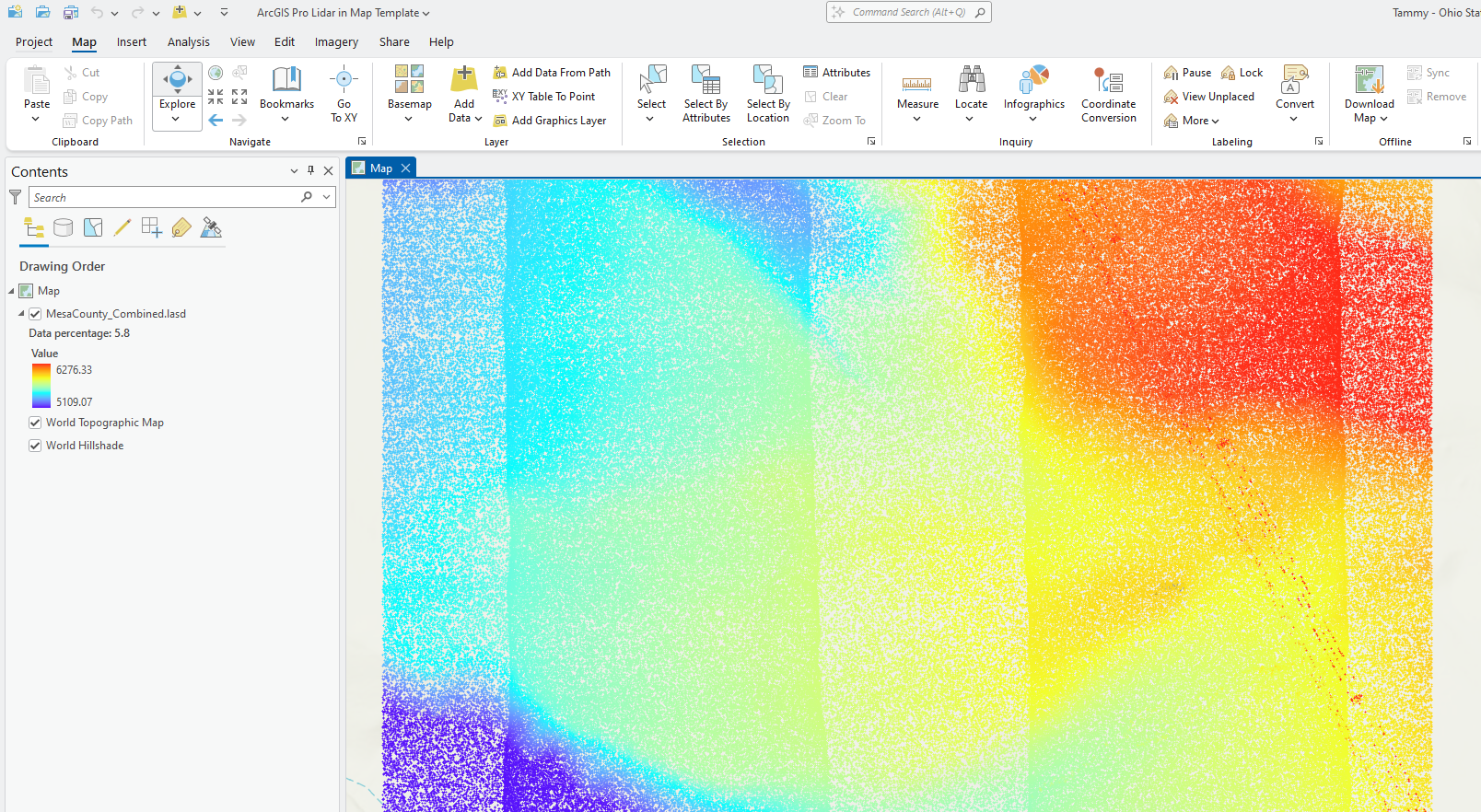
Zoom in and notice how the percentage changes: here the percentage is 5.8 (Figure 15.2), only 5.8% of the point cloud is displayed within the viewer. (Note: Sometimes when displaying percentages of points displayed, an asterisk is used in Contents. This asterisk does change to a % when starting to zoom, the asterisk is just a placeholder at this particular extent.)

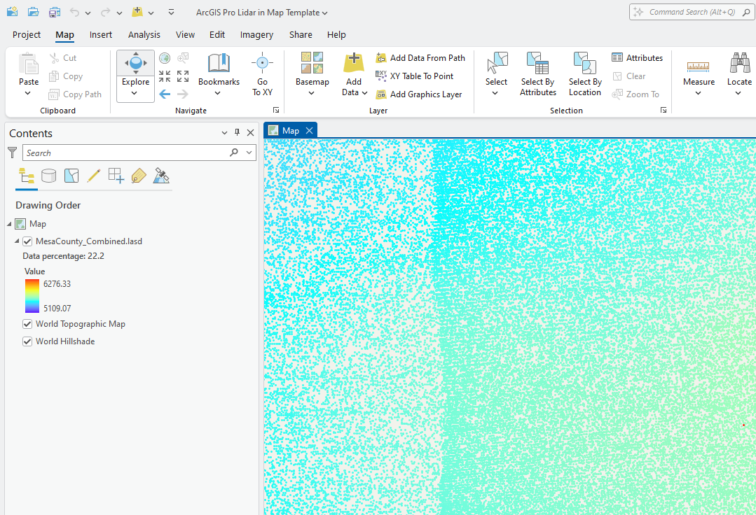
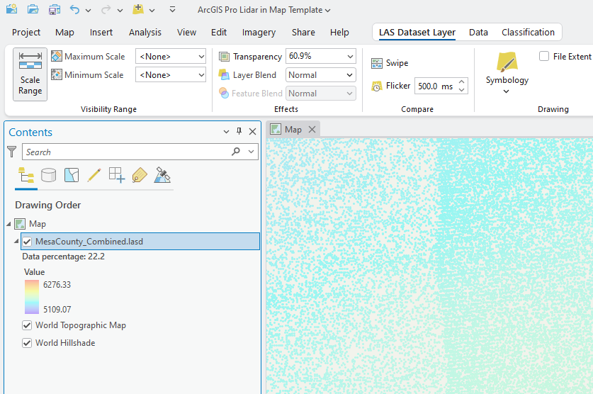
Zoom in again, now it indicates: Data percentage: 22.2 (Figure 15.3).

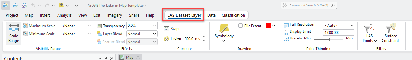
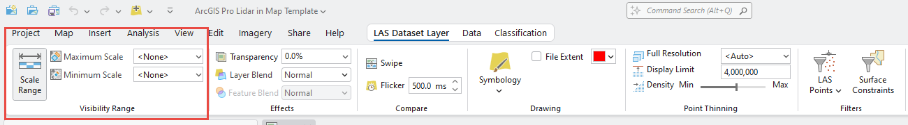
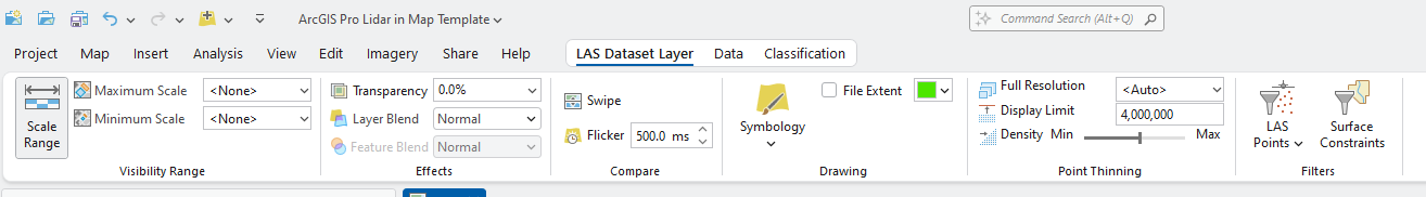
On the ribbon, click on the LAS Dataset Layer tab (Figure 15.4). Here, these display settings can be changed.

On the far left of the ArcGIS Pro® ribbon, in the Visibility Range group, are Maximum Scale and Minimum Scale (Figure 15.5). These controls set the minimum and maximum ranges for the visibility of all the lidar data in the project, including both the footprint and the point cloud.

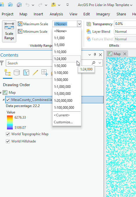
To change the setting from none, click on the down arrow and choose a scale (Figure 15.6). Go ahead and change it and see what happens. Depending on the scale, the footprint or the point cloud may or may not be visible. It also depends on the spatial extent of the data—remember the three Mesa County tiles are only for a very small region.

Go ahead and reset to the default—None.

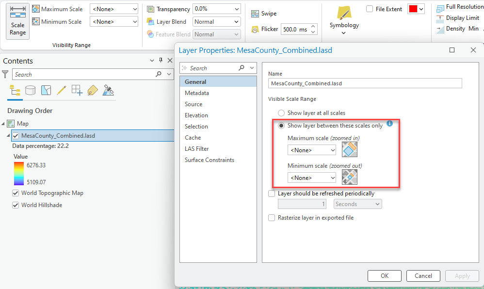
If these settings only apply to one specific lidar dataset, they can also be changed within the Properties of that dataset, under the General tab (Figure 15.7).

Close the Properties dialog and then zoom in so some of the point cloud is visible.

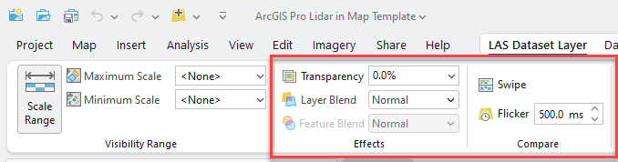
On the LAS Dataset Layer tab, in the Effects and Compare groups are three tools—Transparency, Swipe and Flicker (Figure 15.8).

Transparency allows for “seeing” through the point cloud to view any other data layered below the point cloud. Since the point clouds are not solid for this dataset, not much difference is seen. (Figure 15.9). Reset it to 0%.

A better way to visualize data beneath the lidar data is to use the Swipe tool in the Compare group which uncovers the lower layer—using click and drag with the mouse (Figure 15.10).

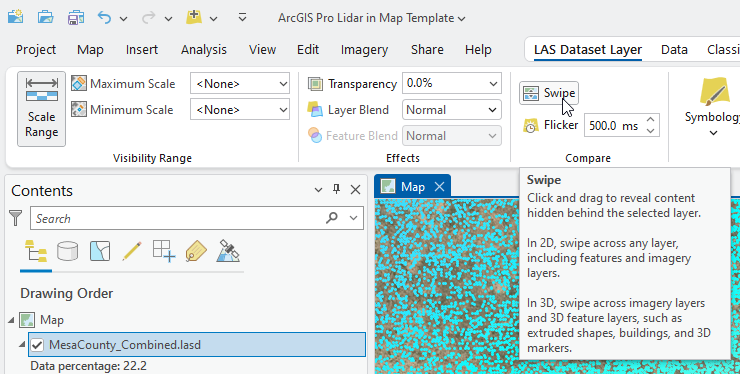
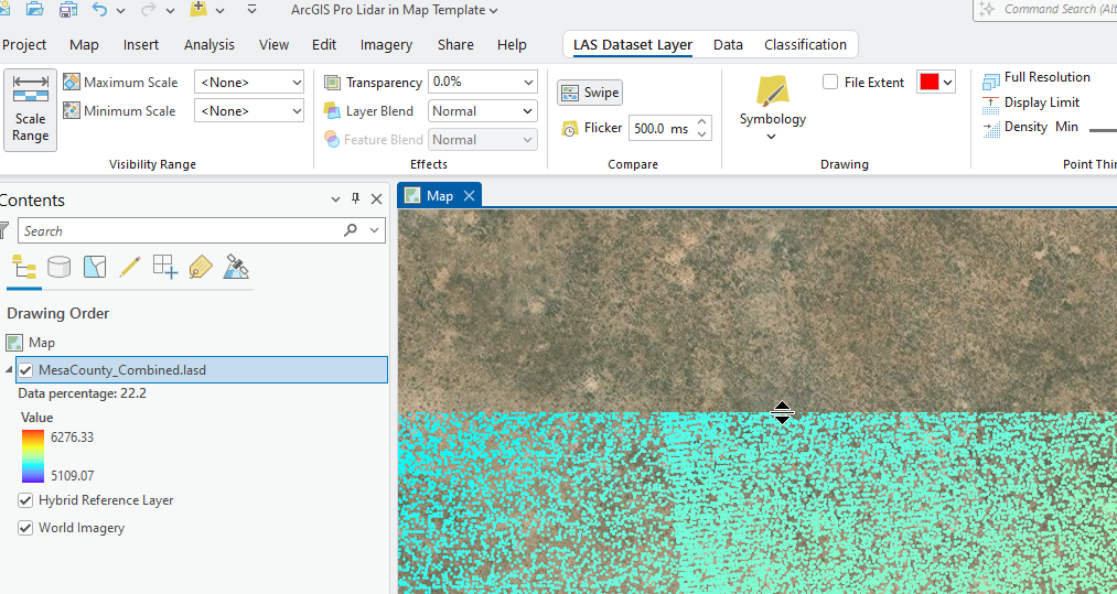
To use Swipe, click Swipe, then move the mouse into the map viewer. A small black upside-down triangle will appear (Figure 15.11). Click and drag the mouse to reveal the layer below the LAS dataset.

The Swipe tool is extremely useful when becoming familiar with a location or when classifying unassigned lidar points.

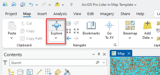
To turn Swipe off, go to the Map tab on the Ribbon and click the Explore button (Figure 15.12).

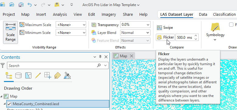
The next tool, Flicker, briefly turns the top layer off and on (Figure 15.13). Flicker is a toggle button, to turn it off just click the button a second time.

In the tool bar, examine the next group to the right—Drawing. Within this group is Symbology and File Extent. Symbology will be discussed in the next chapter.

File Extent controls the color of the footprint. Change it to green (Figure 15.14).

The next set of tools, in the Point Thinning group, controls the display of the entire lidar point cloud—meaning all classifications (Figure 15.15). The settings shown are the default settings for this dataset. Depending on the number of points in the dataset and the density of the points, these settings may be different from .las file to .las file.

The most important of these three settings is LAS Point Density (Figure 15.16).

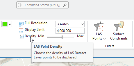
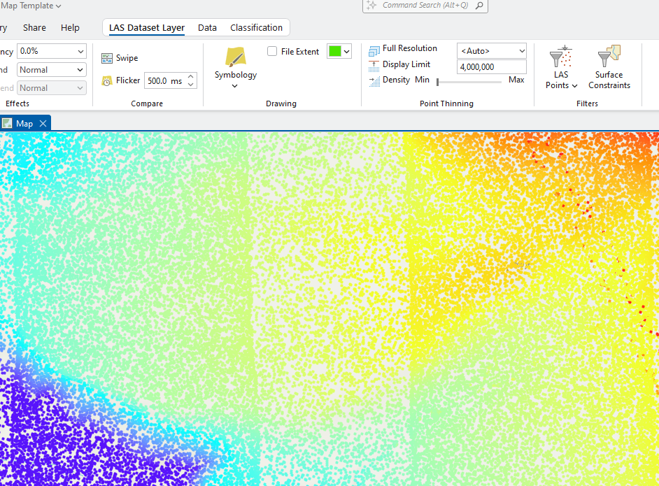
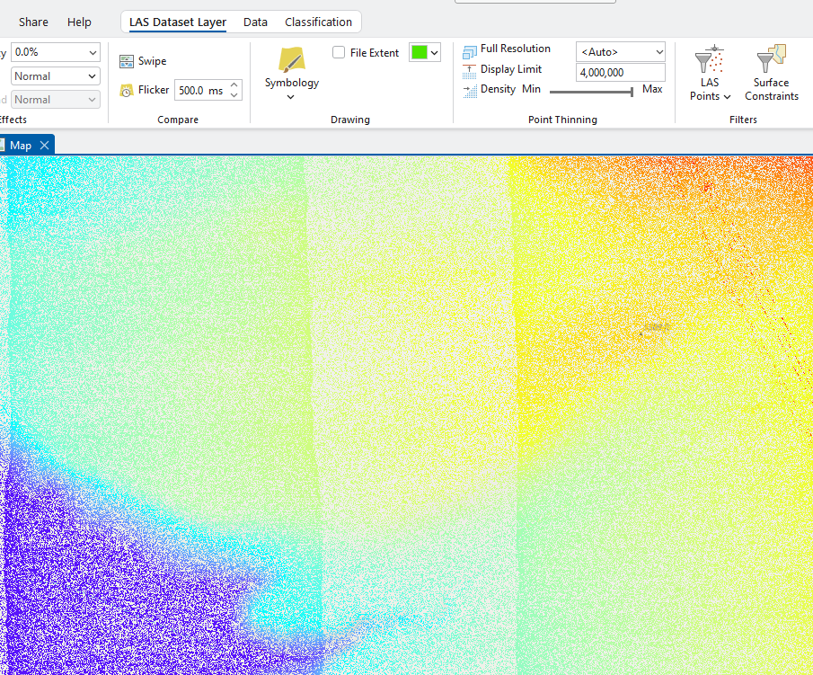
Zoom in to 1:1,000 scale. Then use the slider bar next to Density, going back and forth between Min (minimum) and Max (maximum) to see how it changes the display of the point cloud (Figure 15.17). The points are denser at the maximum setting.

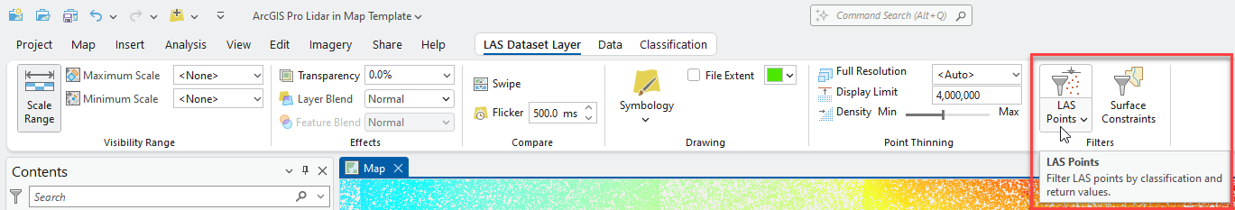
Next is the Filters group and one final example, LAS Points (Figure 15.19). Surface Constraints will be discussed in later chapters.

Click the down arrow, the default is to show All Points (Figure 15.20).

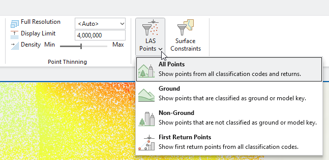
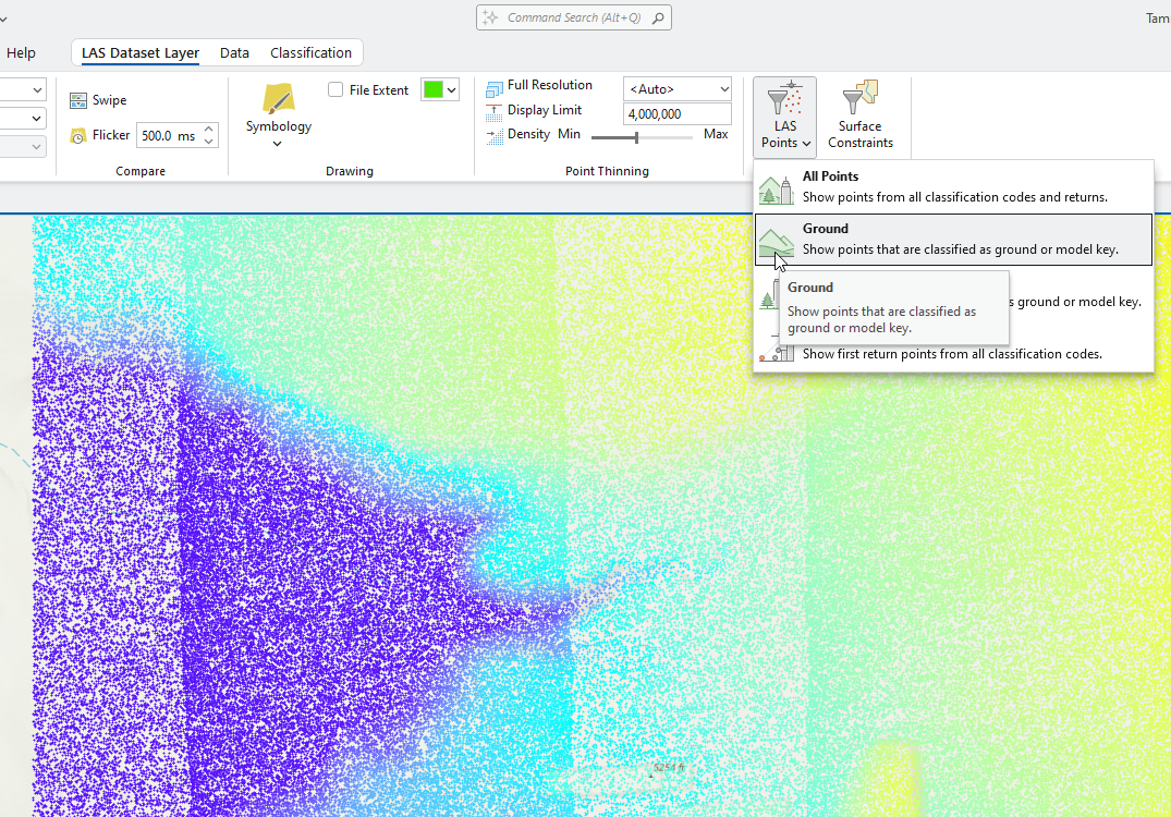
Choose Ground and zoom out to 1:5,000 (Figure 15.21). The only points being displayed are those classified as Ground.

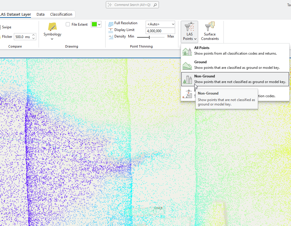
Now chose Non-Ground. For this dataset, that is all of the other points (Figure 15.22).

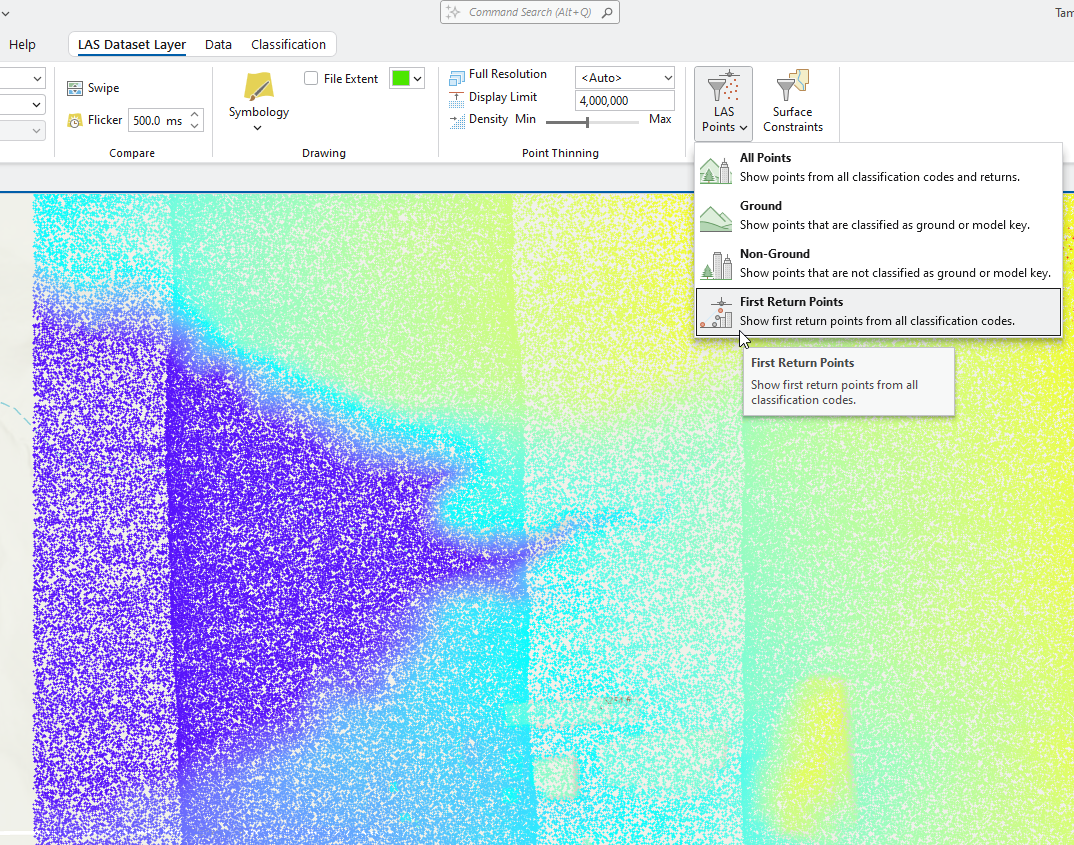
Change to First-Return (Figure 15.23). The first return of a lidar pulse is the first reflection from the pulse that is returned from the sensor, it is typically the highest return in altitude for that specific location. The highest return could be the roof of a building, the top leaf on a tree canopy or the ground if the ground is bare.

Before proceeding, be sure that All Points is selected.

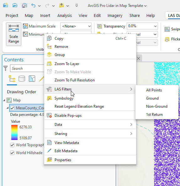
The types of points that are displayed can also be changed in another location. Right-click the LAS Dataset layer and go to LAS Filters. The same options are available (Figure 15.24).

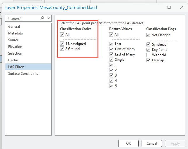
Right-click on the file name again, choose Properties > LAS Filter (Figure 15.25). There is a difference—this method provides more options. Just uncheck the point type to remove it from the display.

Again, the Mesa County lidar data was set up with a Map template—2D only. Please also note that the only classification completed on these data is for ground points.

Close this project and open the San Luis Valley Scene.

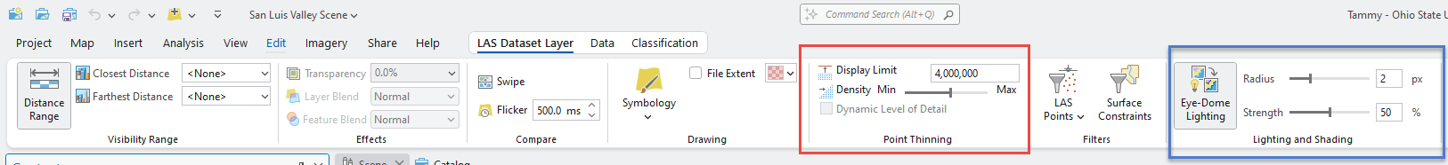
Go to the LAS Dataset Layer tab on the ribbon.  Full Resolution, in the Point Thinning group (red box in Figure 15.26), is not available in a Scene template. All other settings are available and a new group called Lighting and Shading (blue box in Figure 15.26).

Note: If the LAS Dataset Layer tab is not present on the Ribbon, select the layer name in Contents to enable it.

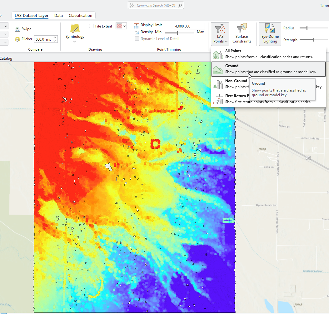
In the Filters group drop down LAS Points and change to Ground  (Figure 15.27).

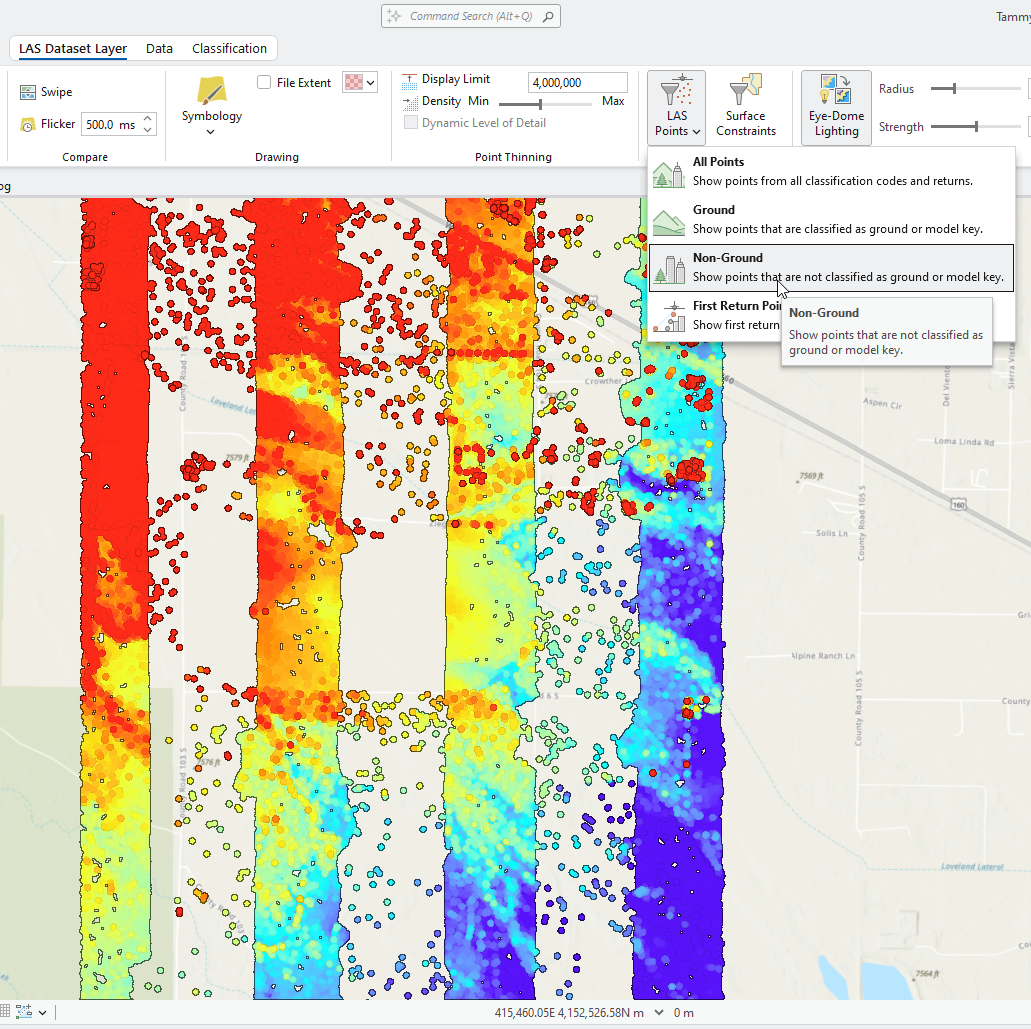
Now change to Non-Ground (Figure 15.28) It appears that the image did not display correctly.

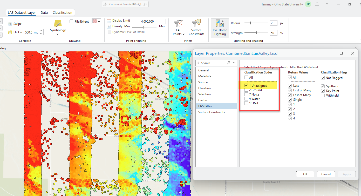
Change the setting back to All Points and then go to Properties > LAS Filter. Uncheck all Classification Codes except Unassigned (Figure 15.29). We will discuss changing the classification in Classifying Lidar Points (Chapters 18-21).

Change the settings at your discretion to see how the different settings change the display (appearance) of the dataset. When finished, be sure to restore to All points.

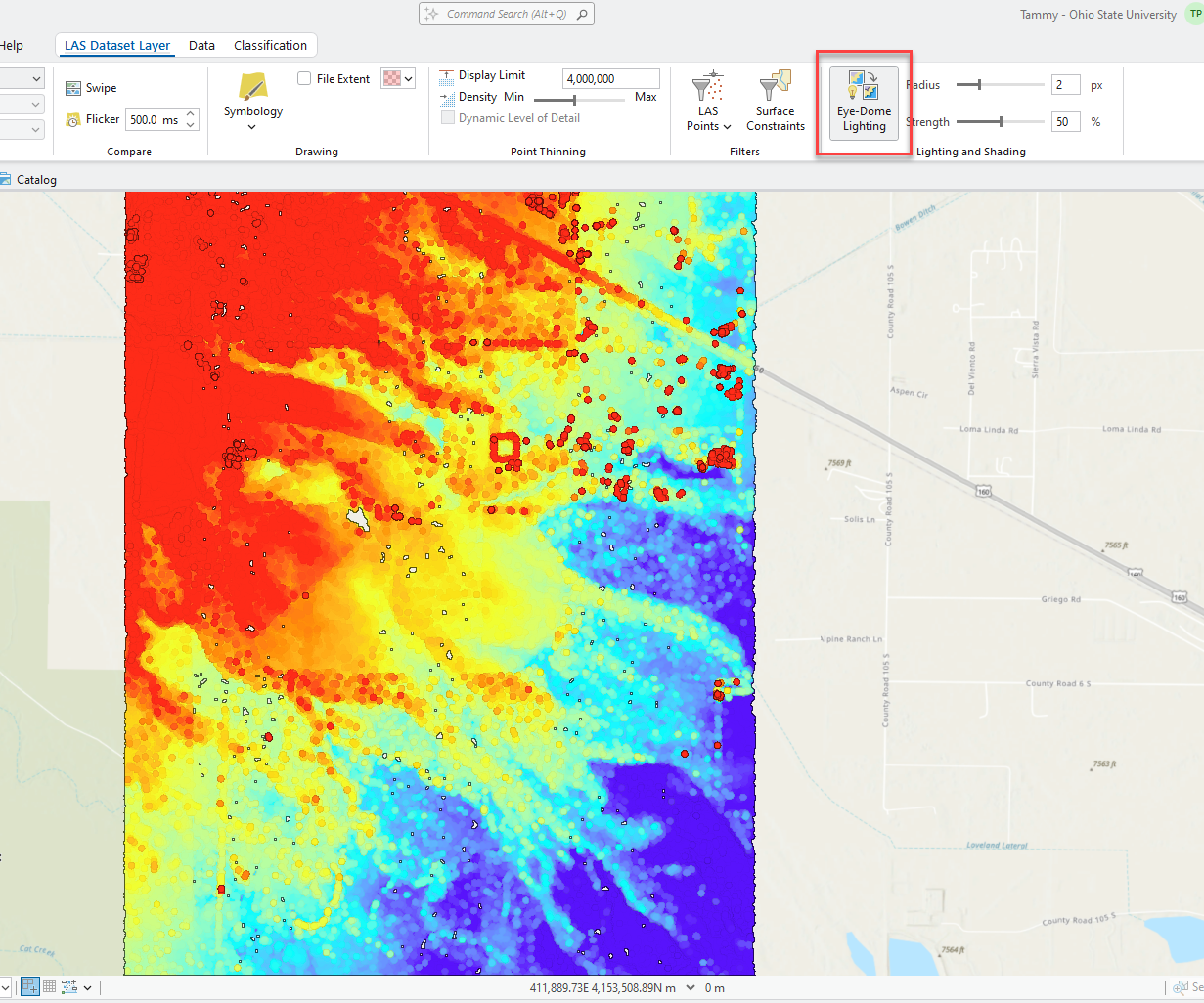
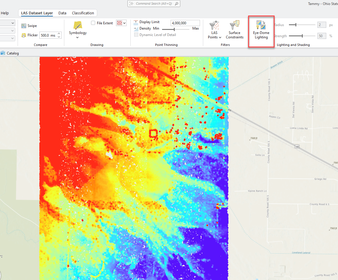
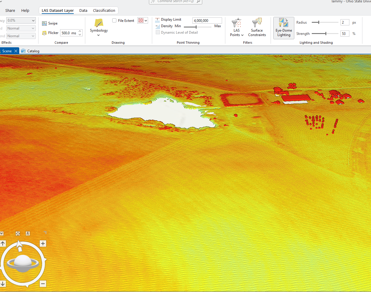
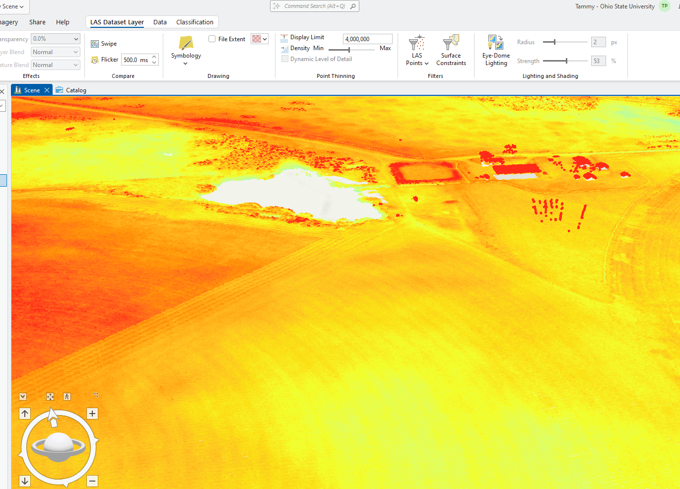
The Lighting and Shading Group is used when viewing in 3-D, so it is only present when setting up a Scene.  Eye-Dome Lighting improves depth perception.  The default is for it to be turned-on (Figure 15.30), and the button is highlighted.   Figure 15.31 shows it turned off.

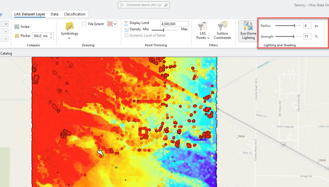
Radius and Strength aid in highlighting the 3-D differences within the viewer (Figure 15.32)

Use the Scene Navigator to look at an oblique view with Eye Dome Lighting turned on (Figure 15.33) and turned off (Figure 15.34).  These settings aid in viewing only, they do not change the point cloud values.

Please change the settings at your discretion to see how the different settings change the display (appearance) of the dataset. When finished, be sure to restore the defaults.

The next chapter, Chapter 16. Lidar Symbology, discusses changing the symbology of the point cloud.