Chapter 13. Combining Tiles into One .lasd Dataset

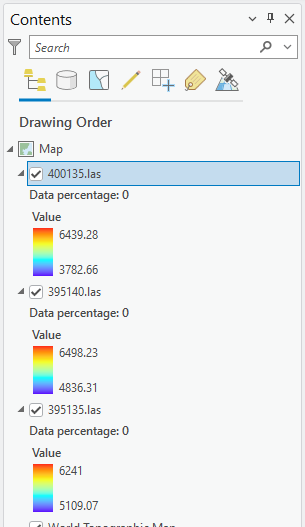
Chapter 10. Setting up ArcGIS Pro for Lidar Data introduced two project templates for adding .las tiles. In that chapter, multiple tiles were added to a map project and displayed as separate data files. Recall that the symbology displayed in the map viewer demonstrated different stretched values (Figure 13.1).

This chapter will demonstrate how to create one data set from multiple lidar tiles.

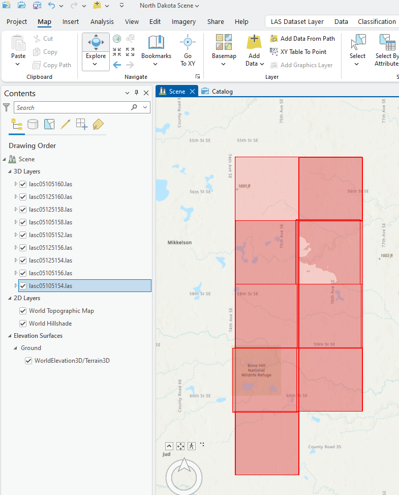
Open the North Dakota project that was created in Chapter 10. Setting up ArcGIS Pro for Lidar Data. Recall that the North Dakota lidar project map was created using Local Scene (3D) as the template (Figure 13.2).

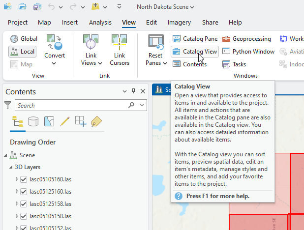
Open Catalog View (Figure 13.3).

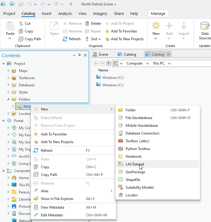
Once Catalog View is open, right-click the project’s folder, then New and choose New LAS Dataset (Figure 13.4).

A file called New LAS Dataset (.lasd) is created (Figure 13.5).

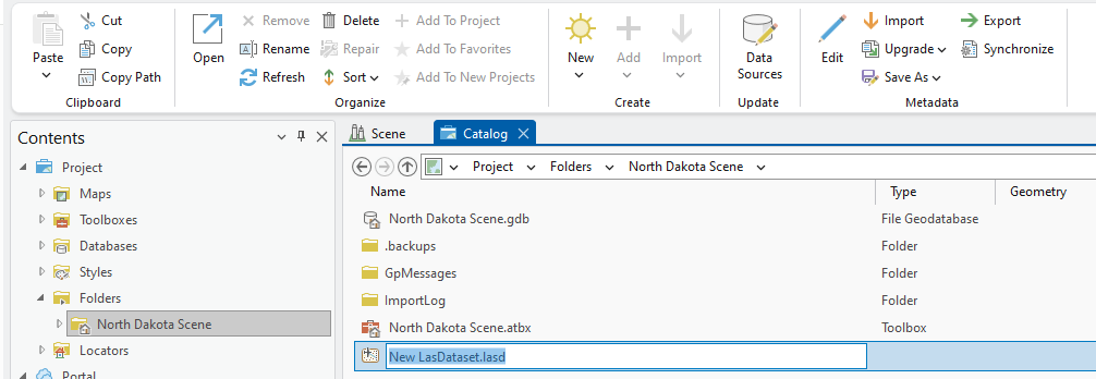
Right-click New LAS Dataset.lasd and Rename to “ND_James_River_Combined”.

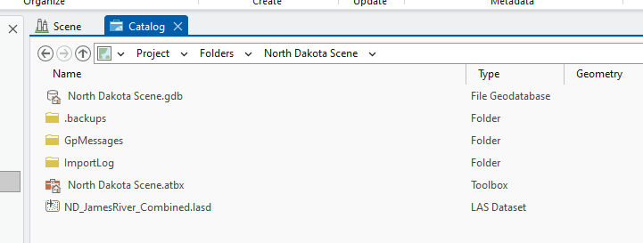
The file may initially appear to disappear. You may need to give the ArcGIS Pro® software a moment to rename and redisplay the file (Figure 13.6).

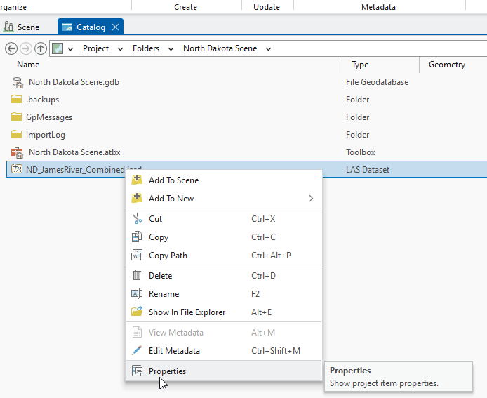
Right-click the ND_James_River.lasd  file and choose Properties (Figure 13.7).

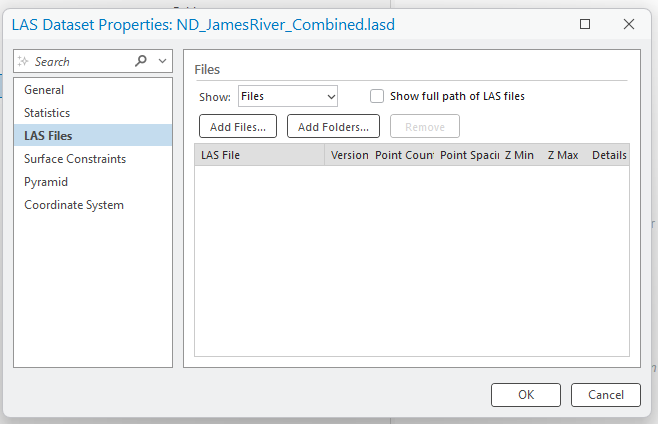
The Properties dialog opens (Figure 13.8). Right now, the dataset is empty, so no information is available.

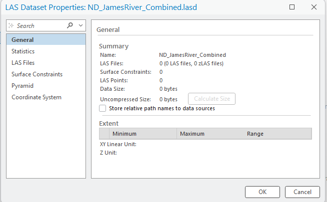
Select LAS Files on the left (Figure 13.9)—the data will be added here.

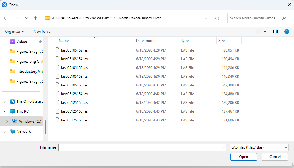
Choose Add Files and navigate to the North Dakota James River tiles (Figure 13.10).

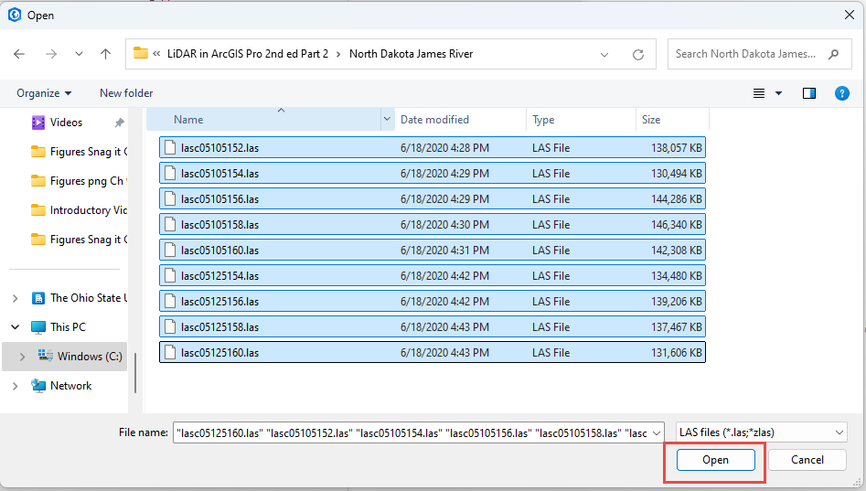
Choose all the .las tiles for North Dakota then click Open (Figure 13.11).

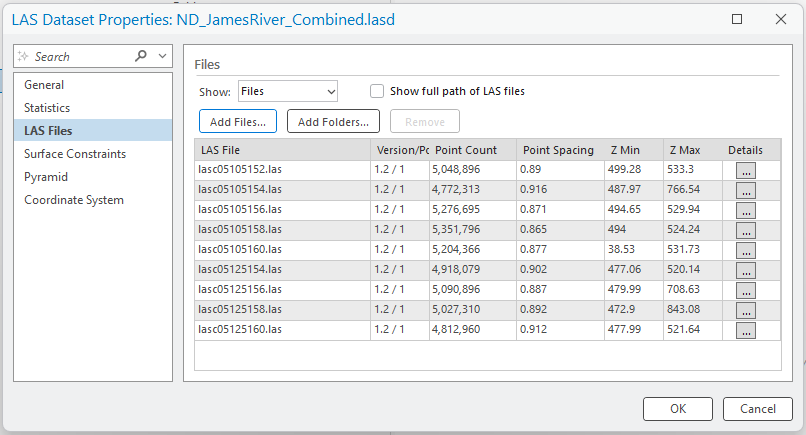
All the files are now populated in the dialog (Figure 13.12). For the first tile in the list (lasc05105152.las), go to the end of the row and click the ellipsis (…) under the Details column.

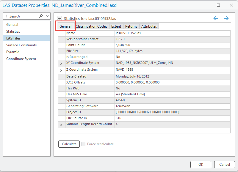
Statistics for the .las file opens. Selecting the General tab in in the right pane (red box, Figure 13.13), reveals statistics for this individual dataset (not all nine that were added) (Figure 13.13).

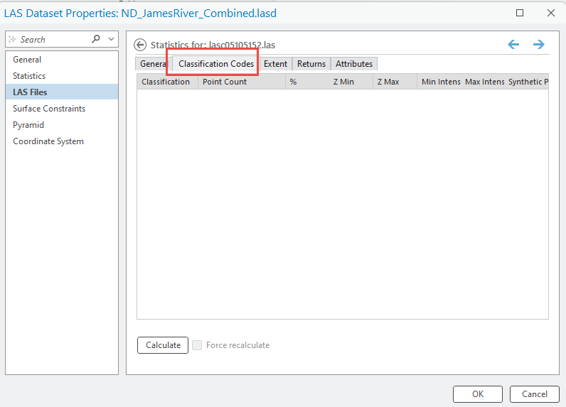
No information appears in the other tabs (Figure 13.14 is one example under Classification Codes).

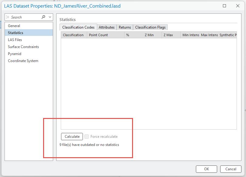
Select Statistics in the left pane (Figure 13.15). It is empty because Statistics have not yet been calculated. Click Calculate at the bottom.

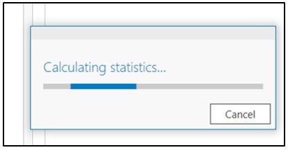
A processing dialog opens (Figure 13.16).

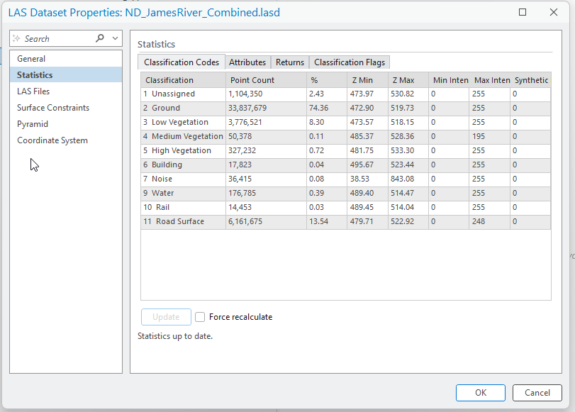
When finished, statistical information is displayed—this tab is statistics for all nine tiles (Figure 13.17). It notes how many points are classified as Ground, as Low Vegetation, etc., or how many are Unassigned to any classification category. Classification is covered in subsequent chapters.

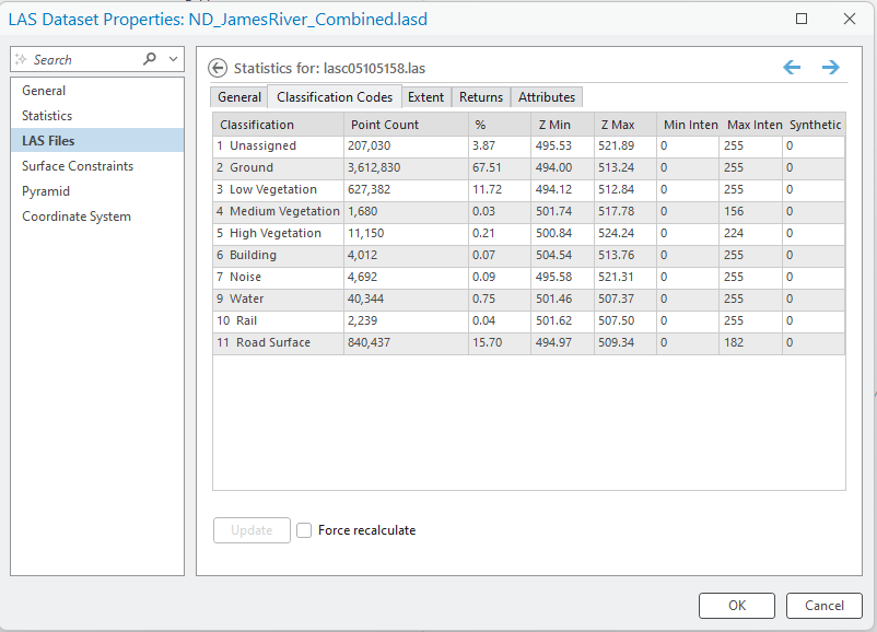
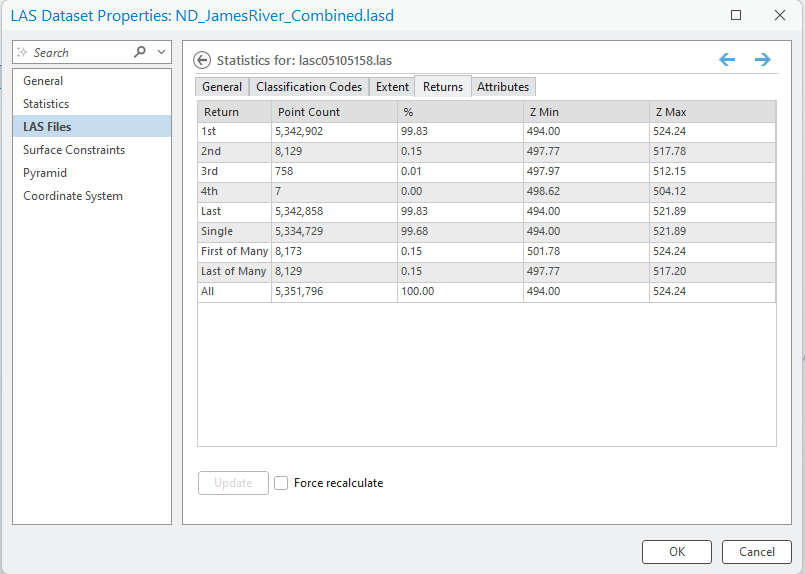
To view the statistics for any one tile, go back to LAS Files and select the ellipsis (…) under Details (Figures 13.18 – shows Classification Codes and 13.19 shows Returns—the type of return). This information will be extremely important in learning lidar tools in subsequent chapters.

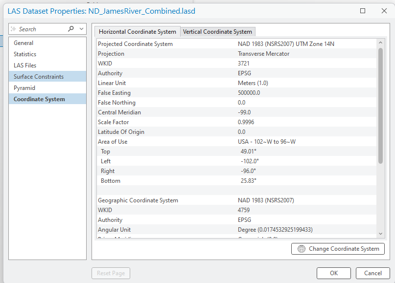
Go to Coordinate System on the left (Figure 13.20). The coordinate system information has been incorporated and read from the individual tiles. Please note, this is another reason to completely review all metadata once the lidar tiles have been downloaded. If trying to combine tiles with different coordinate systems, an error will occur. Once finished reviewing all the data, click OK to finish creating the newly combined data set.

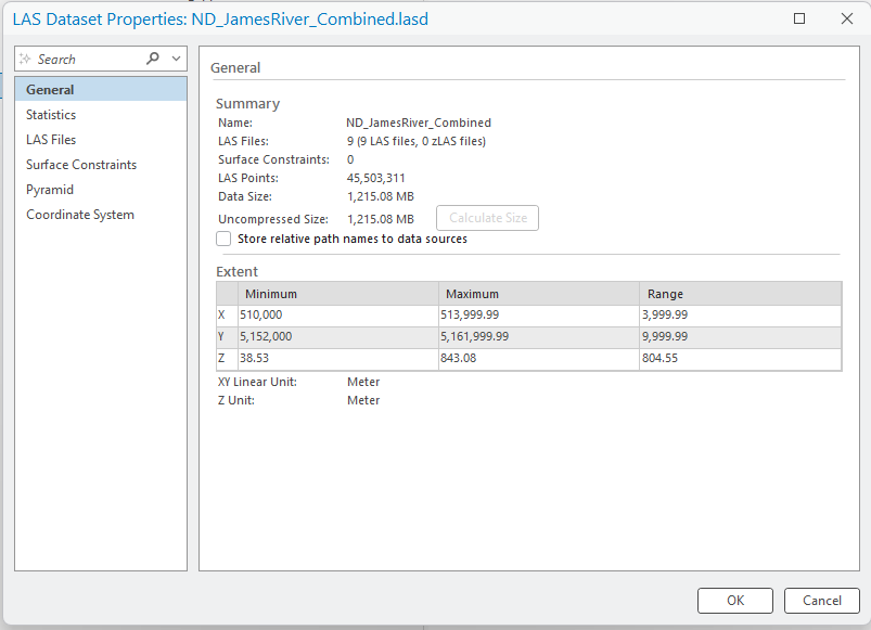
It does not look like anything occurred. But right-click again on the new dataset and go to Properties, the data has been saved. All the tiles are now combined (Figure 13.21).

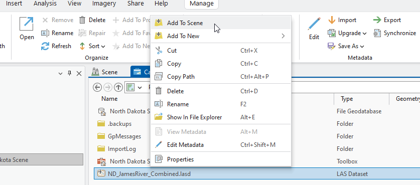
Now right-click on the data set and choose Add to Scene (Figure 13.22).

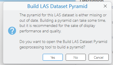
If you receive the following message, click Yes (Figure 13.23).  It will take you to the geoprocessing tool Building LAS Dataset Pyramid dialog.  Once that window opens, click Run, there is no need to change any of the default settings in that geoprocessing tool.

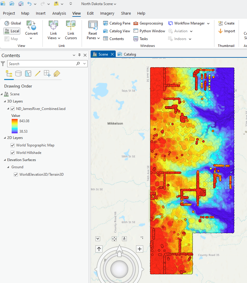
Then at the top of the viewer, click on the Scene tab to change from Catalog View. (Figure 13.24). The new combined file and all the individual tiles are within the scene.

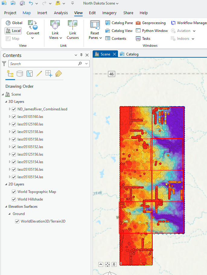
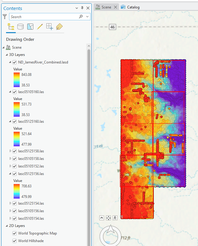
Not sure if things changed? Uncheck the new dataset in Contents to see the individual tiles underneath. The individual tiles have their own individual stretched values and the individual tiles are distinguishable from each other in the map viewer, whereas all the symbology is stretched over the entire range of values for the new .lasd dataset. (Figure 13.25)

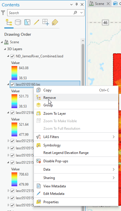
To remove the individual tiles, right-click on each tile and choose Remove (Figure 13.26). Only keep the newly created ND_James_River_Combined LAS dataset.

Expand the symbology in Contents and Save the project (Figure 13.27).

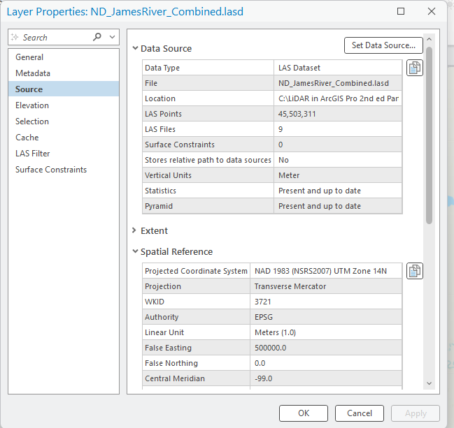
Right-click on the file name and go to Properties. This metadata was created when statistics was calculated.  Thus, it is not necessary to go to Catalog to find spatial reference and classification information. (Figures 13.28 and 13.29)  The classification information will be important in subsequent chapters.

You have just merged lidar data points from individual .las files (tiles) into a single .lasd file (LAS dataset). Note that there are other techniques that can be conducted to create a single .lasd file from multiple files.

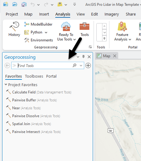
Re-open the Mesa County Project created in Chapter 10. Setting up ArcGIS Pro for Lidar Data. Then click on the Analysis tab and select Tools to open the Geoprocessing dialog (Figure 13.30).

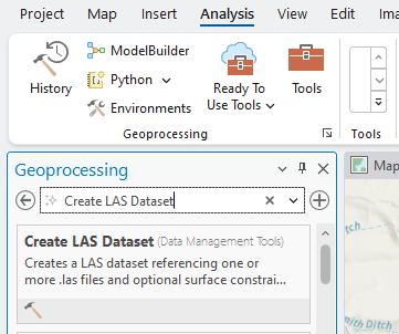
Under Find Tools, search for “Create LAS Dataset” (Figure 13.31).

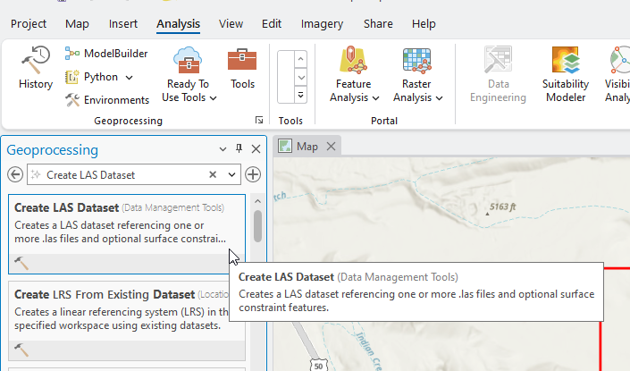
Select the first option—Create LAS Dataset (Data Management Tools) (Figure 13.32.)

Select Create LAS Dataset to open it (Figure 13.33).

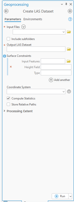
For Input Files, select the drop down arrow at the end of the line and select the three Mesa County lidar tiles from Contents.  Alternatively, open the folder at the end of the line and navigate to the three Mesa County Colorado lidar tiles (Figure 13.34).

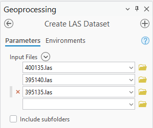
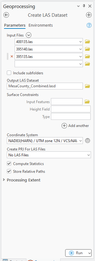
The three files have populated under Input Files. Under Output LAS Dataset, name the file. Please note that the new LAS dataset file is automatically saved into the project folder (Figure 13.35). Be sure to check the boxes in front of Compute Statistics and Store Relative Paths. Leave all other inputs as default (or blank). Note: By selecting Relative Paths, the software will establish a path to the data that is relative to the location of the ArcGIS Pro® project. If you have all of your data and project information in one folder and transfer the entire folder, you will not end up with red exclamation points resulting from undefined data paths.

Then at the bottom of the Create LAS Dataset dialog, click Run (Figure 13.35).

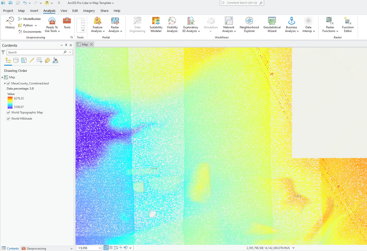
When the tool is finished running, the new .lasd file (LAS dataset) appears in Contents and is automatically added to the scene (Figure 13.36).

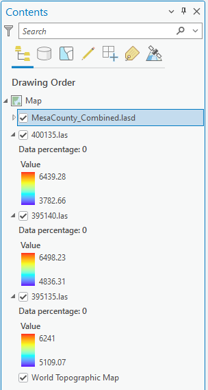
Remember, the point clouds might not be displayed until zoomed in (Figure 13.37).

Need verification that the files were combined? Figure 13.37 shows the uncombined .las files are unchecked in Contents.

Right click on each of those individual tiles and Remove them so that only the new combined file is present (Figure 13.38).

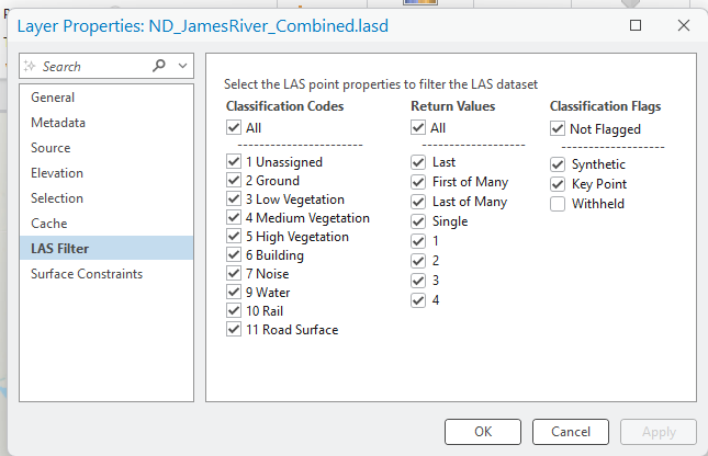
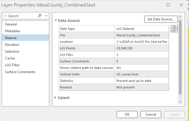
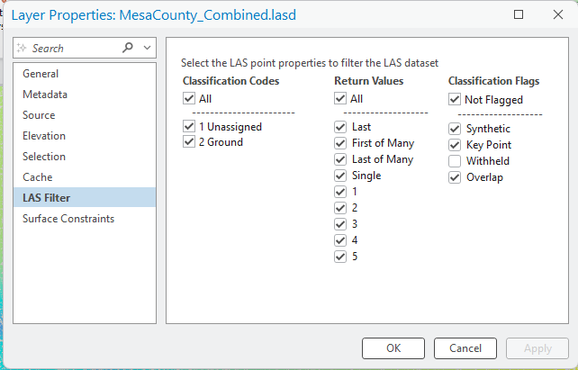
Right-click on the new file and check the Properties, including Source (Figure 13.39) and LAS Filter (Figure 13.40) .

Save the Mesa County project and go to Project at the top left. Create a new Local Scene project and name it  “San Luis Valley Scene”.

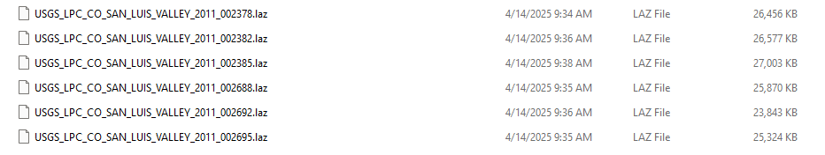
Recall from Chapter 8. Lidar and the National Map Viewer, the San Luis Valley Colorado tiles downloaded are in LAZ format (Figure 13.41).

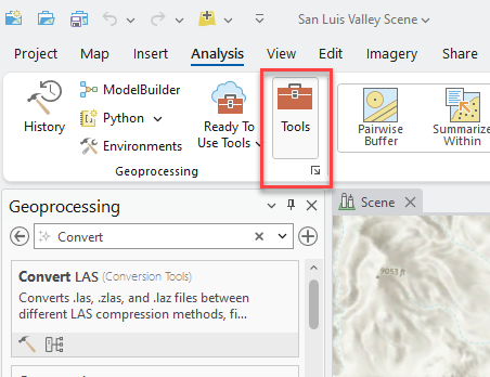
ArcGIS Pro cannot display data in LAZ format but we can convert LAZ to .las within the software.  In the San Luis Valley Scene, click on Analysis and then Tools (red box).  Search for “Convert LAS” (Figure 13.42).

Open the tool (Figure 13.43).

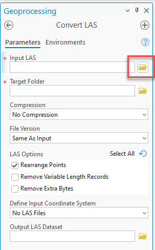
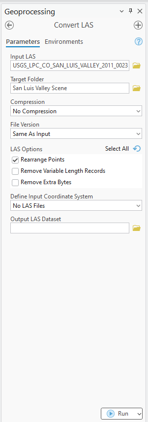
Use the file folder at the end of Input LAS (red box in Figure 13.43) to navigate to the local folder where you saved the LAZ files downloaded from The National Map in Chapter 8. Lidar and the National Map Viewer.  Target Folder is where you want to save the new .lasd file, and you do not need to name an Output LAS Dataset, the new .las file will maintain the original file name. Run the tool (Figure 13.44).

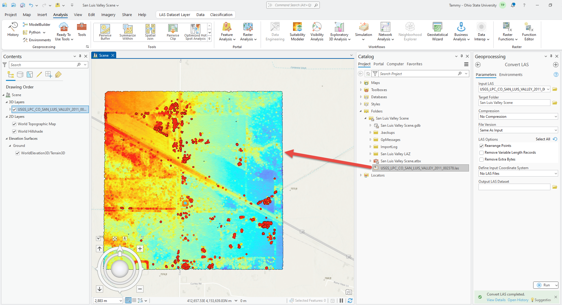
Once the tool is finished, it looks like nothing happened because there is no file in Contents.  But if you look in the Catalog pane, a .las file has been created (if you don’t see the file, right-click on the file folder name and click refresh).  In the Catalog pane, click on the file name and drag it into the scene (Figure 13.45).

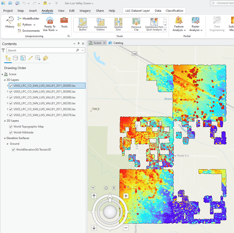
Please complete this process for each of the other five downloaded San Luis Valley LAZ files. When finished, your San Luis Valley Scene will look similar to Figure 13.46.

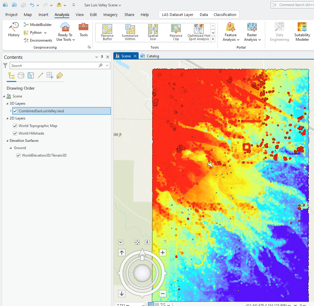
Now combine all these new files into one dataset.  Use either of the methods outlined previously.  When you are done, remove the individual files and your San Luis Valley Scene should look similar to Figure 13.47.

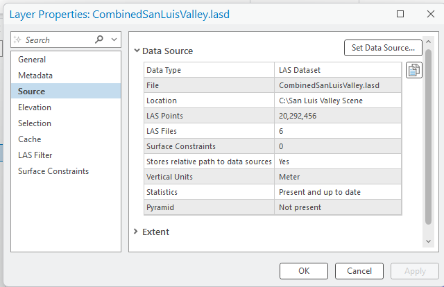
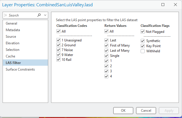
Right-click on the file name, go to Properties, check Source (Figure 13.48) and LAS Filter (Figure 13.49) to see the classification codes. Source shows that there are six LAS files in this combined dataset and that the Statistics are Present and up to date.

Save and close the project.

This concludes this chapter. Subsequent chapters will review changing the display settings, including changing the percentage of the point cloud that displays automatically when zooming in and out, and when displaying certain classes, return values or classification flags.

Later chapters will provide instruction on classifying unassigned points, adding surface constraints and creating a digital elevation model.