Chapters 1 – 6 introduced ArcGIS Pro® basics using vector files. Chapters 7 – 9 introduced locating and downloading lidar data and reading the metadata that always accompanies lidar data. This chapter introduces the use of ArcGIS Pro with lidar data and the two project templates that can be used—map or scene. In this chapter, the lidar data previously downloaded is added and displayed in ArcGIS Pro®, and navigation tools are introduced. The next chapter will discuss additional ArcGIS Pro® tools for lidar datasets.

Opening ArcGIS Pro® using a Map Template

Chapter 1. Creating a New Project provided instructions on using vector files in a new project with a Map template. Map templates are two-dimensional (2D) representations of data. A Map template can be used to display lidar data, but it limits processing and display options strictly to 2D.

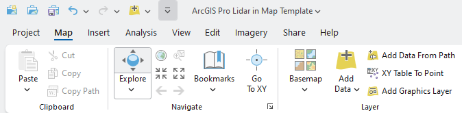
Open a new project using a Map template^[1]. Go to the Map tab and click on Add Data in the Layer group(Figure 10.1).

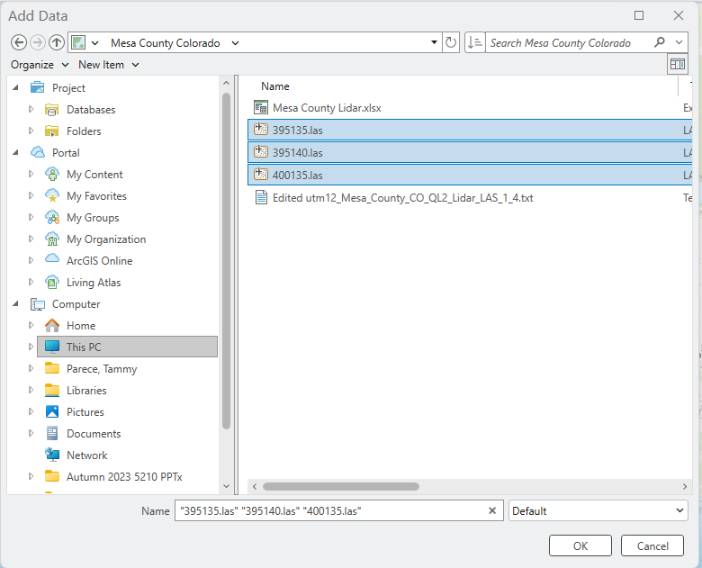
In the Add Data window, navigate to the folder with the lidar data for Mesa County, Colorado, and add all three Mesa County Colorado LAS files (Figure 10.2).

As when vector files are added, the map project zooms to the location of the data. Three new tabs appear on the Ribbon—LAS Dataset Layer, Data, and Classification. Those tabs are discussed in subsequent chapters.

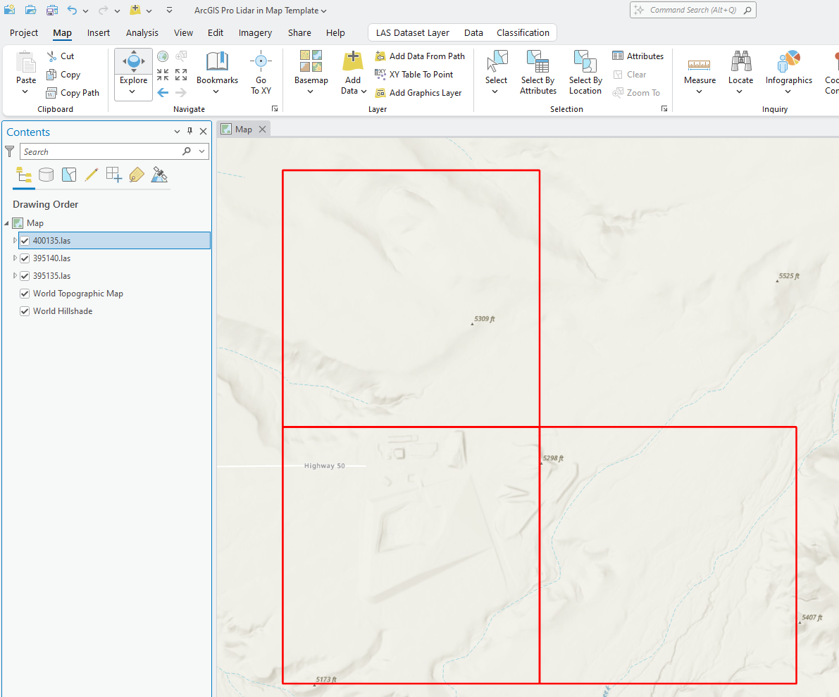
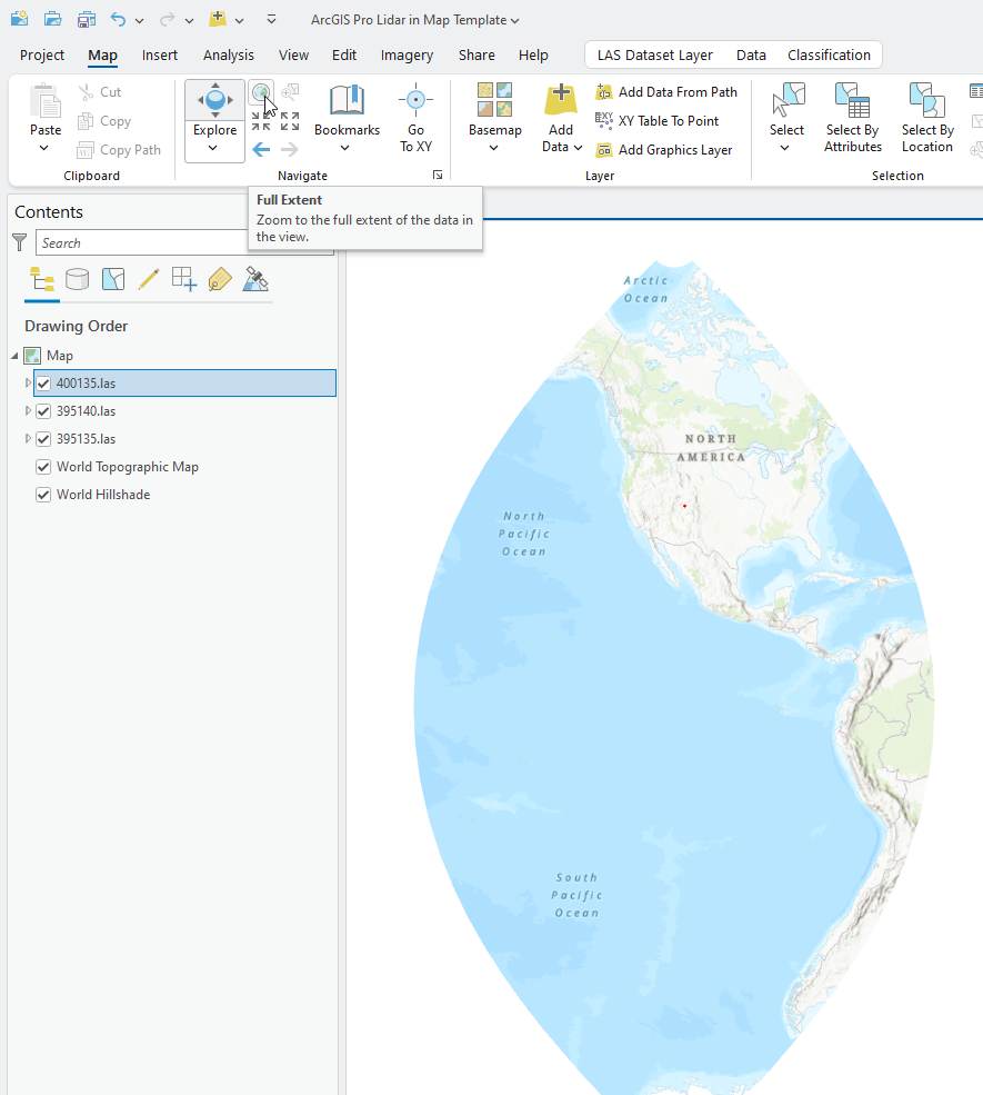
All that is displayed in Figure 10.3 are red lines, so where is the data? Because lidar data files are large, even when covering a small area, ArcGIS Pro® may only show the footprint of the lidar tiles at full extent.

With ArcGIS Pro®, the mouse wheel allows zooming in (forward) and out (backward). See Figure 10.4 for mouse functionality.

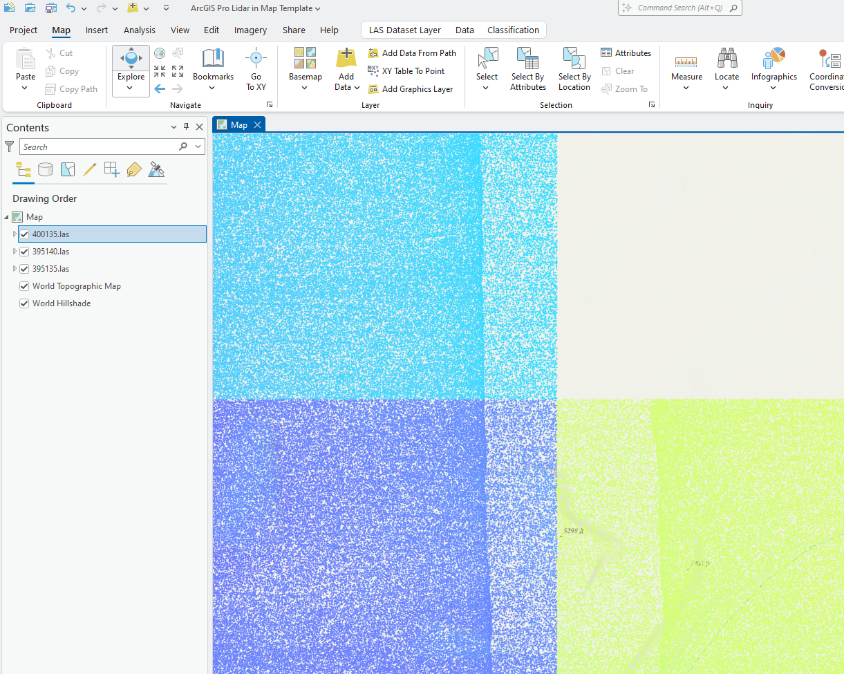
Use the mouse wheel to zoom in, and the individual data points will begin to display (Figure 10.5). Due to the size of the LAS files, ArcGIS Pro® does not display all of the points. This setting can be changed and will be discussed in subsequent chapters.

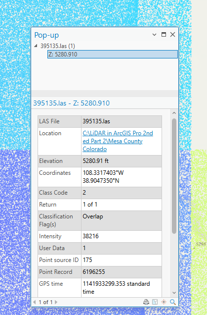
The left mouse button allows for identifying and panning. To identify, click anywhere in the lidar point cloud and a Pop-up appears(Figure 10.6). The Pop-up can be resized to display all attributes for a specific point.

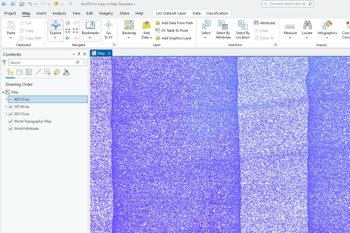
To pan, drag (left mouse button) while the pointer is anywhere in the map viewer. An example of a new location is shown in Figure 10.7.

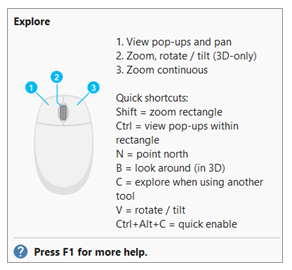
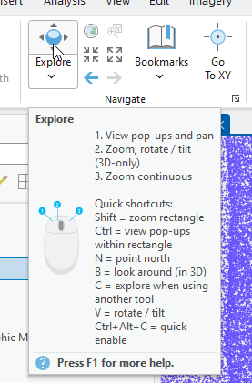
Navigating within the map viewer can also be accomplished with Explore, found in the Map tab on the ribbon. Hovering over Explore also provides details on navigating with the mouse and using shortcut keys on the keyboard (Figure 10.8). Practice with the Explore button, the shortcut keys, and with the mouse. The only functionality at this point is 2D, so rotate/tilt and look around (in 3D) don’t work in the Map template.

Be careful when using the right mouse button—Zoom continuous—because ArcGIS Pro® will zoom in quite rapidly, appearing as if the data disappeared. If this happens, use the mouse wheel to scroll out. Don’t hit the full extent button, it will zoom to the full extent of the base map (Figure 10.9).

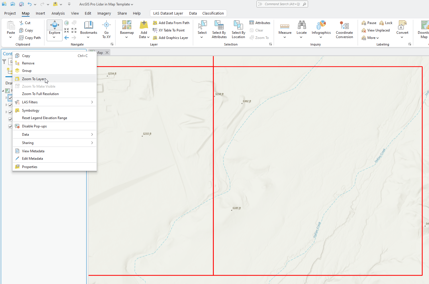
If the full extent button was clicked, don’t panic. Right-click on any of the .las files in Contents and choose Zoom to layer (Figure 10.10).

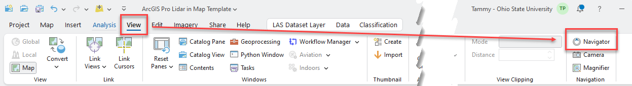
Next, go to the View tab on the Ribbon to find the Navigator button in the Navigation group (Figure 10.11).

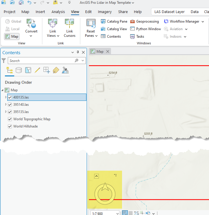
Clicking on Navigator places a navigator option in the map viewer (yellow highlighted in Figure 10.12).

The pointer on Navigator always points towards North (blue arrow in Figure 10.13).

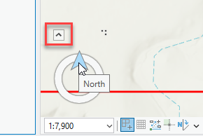
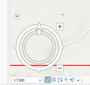
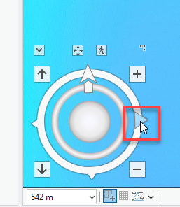
Click on the small up arrow on the left side of Navigator (red box in Gigure 10.13) to reveal additional functions (Figure 10.14).

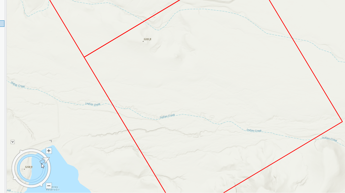
Drag the box on the inner circle (just below the North Pointer) to the right to rotate the image to the east (Figure 10.15).

Go ahead and practice with Navigator. Rotate back and forth. The plus and minus buttons are zoom in and zoom out. While functionality is limited in 2D, the Navigator tool will be the primary navigation source when working in three dimensions (3D).

To remove Navigator, click Navigator again in the toolbar. Be sure to point your map back in the North direction by moving the north arrow or using the shortcut Shift-N.

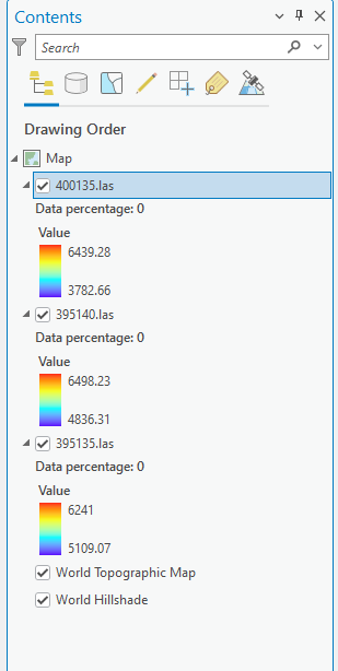
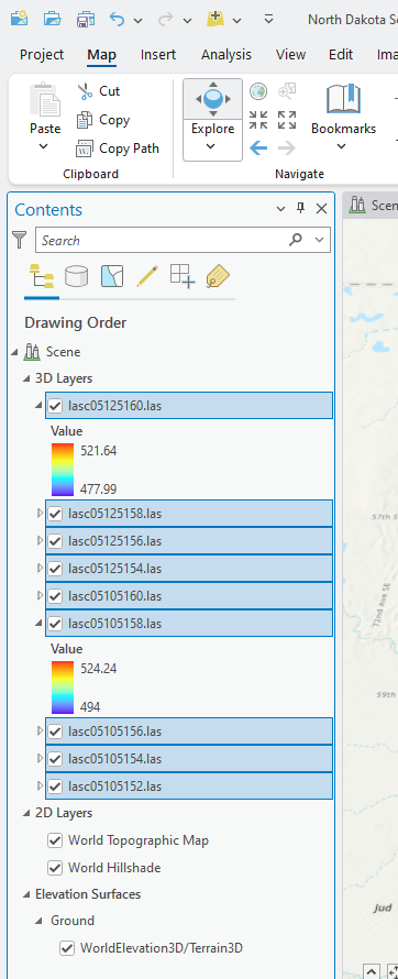
When the tiles were first added, the symbology for each tile was collapsed in the Contents pane (Figure 10.16).

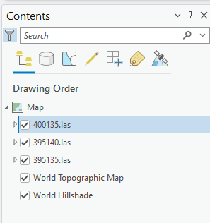
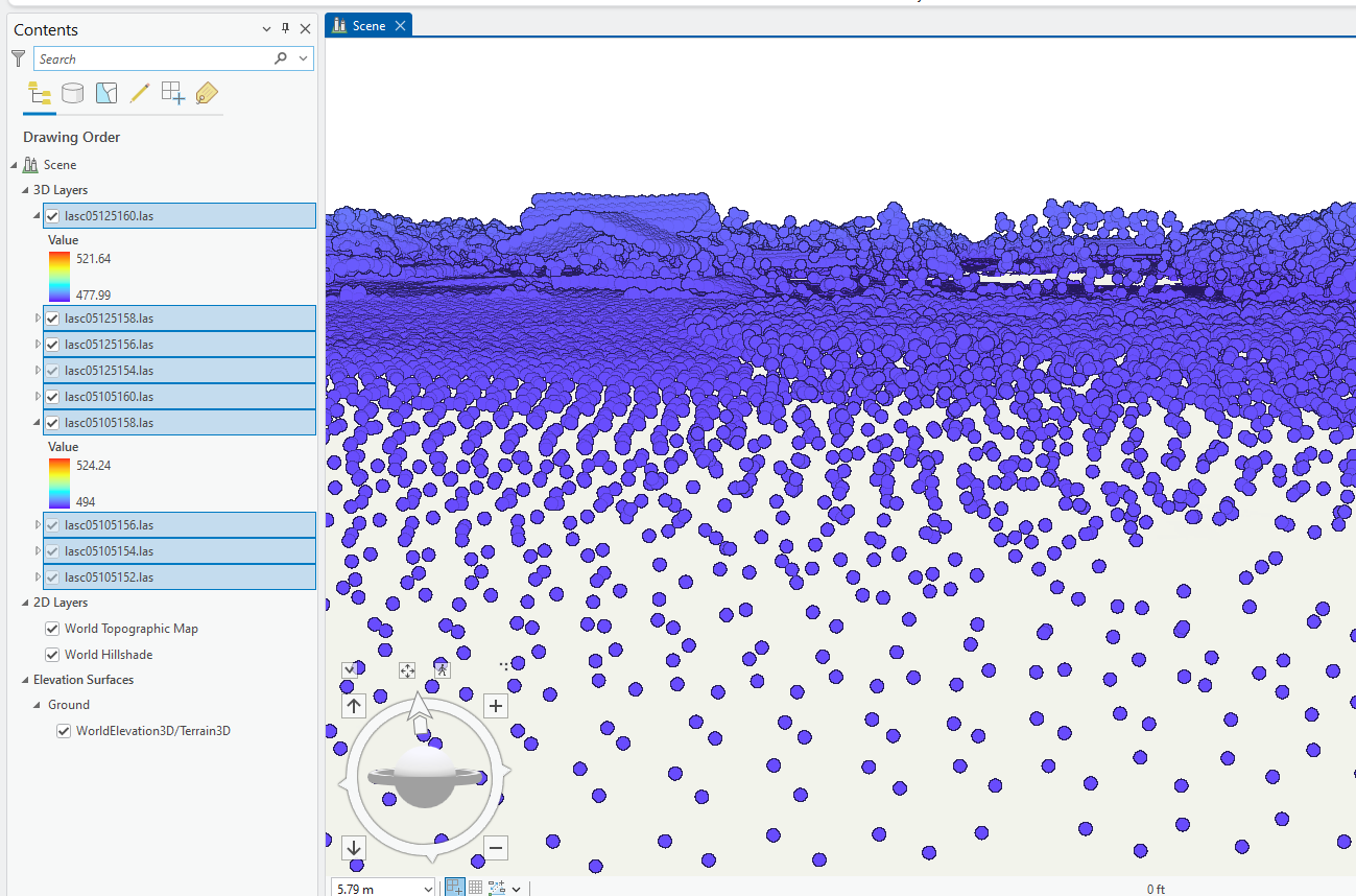
Expand the symbology. The symbology is the stretched type, but each .las file has a different range of values (Figure 10.17).

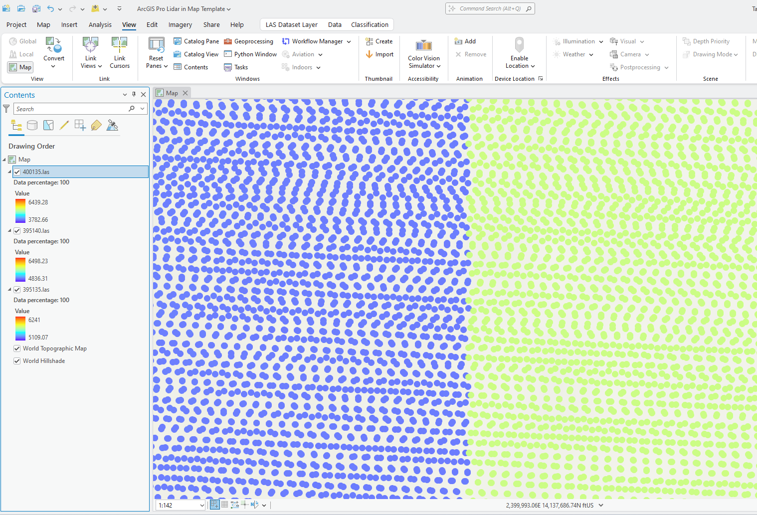
Zoom in to one of the boundaries between two tiles. Because the tiles are separate and the values within each tile vary, the symbology does not exactly match, and when viewing the point cloud, the two tiles are distinct. (Figure 10.18).

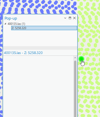
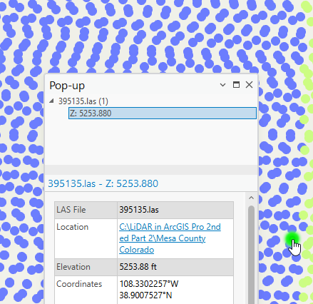
Use the identify pop-up to look at two points right next to each other—choose a point in one tile and the other point in the neighboring tile. In Figures 10.19 and 10.20, the two points next to each other (one in one lidar tile and one in the other), are very close in value— 5258.320 feet and 5253.880 feet. The next chapter will demonstrate how to combine multiple tiles to avoid this symbolization disparity.

This concludes the instruction on lidar using the Map template. As a reminder, a Map template is 2D only. Lidar’s most beneficial aspect is 3D. Why use a Map template with only 2D? Using a Map template is beneficial when becoming familiar with data or determining if the data downloaded covers the precise area of interest, among other reasons. Save and close the project.

Lidar and a Scene template

For this section, use the North Dakota lidar data downloaded in Chapter 7. Locating Lidar Data.

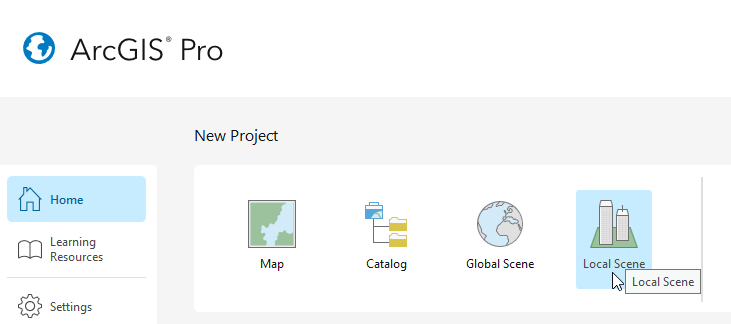
Create a new project using the Local Scene template (Figure 10.21). Name the project and identify the Location, similar to creating a new project using a Map template.

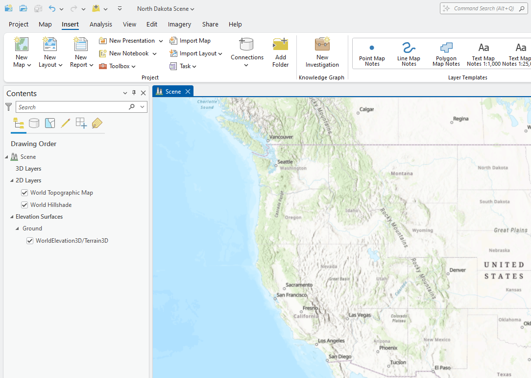
The first difference from a Map template is in Contents. 3D Layers, 2D layers, and Elevation Surfaces are included as default layer groups (Figure 10.22)

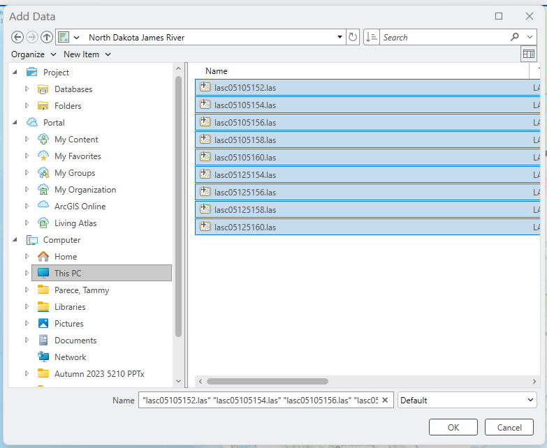
Click on the Map tab and Add Data. Add all nine lidar tiles from North Dakota (Figures 10.23 and 10.24).

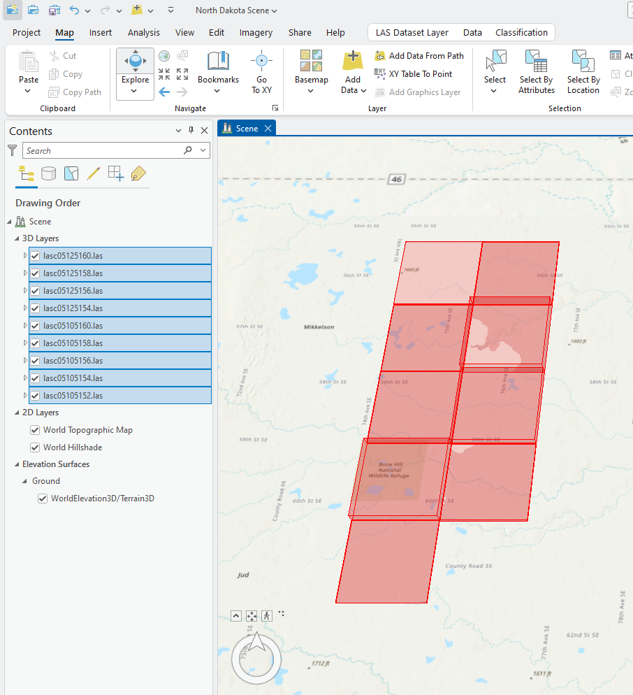
The North Dakota tiles look very different from the Mesa County Colorado tiles. Each lidar acquisition is different depending on the project. This is why metadata must be examined before using the data.

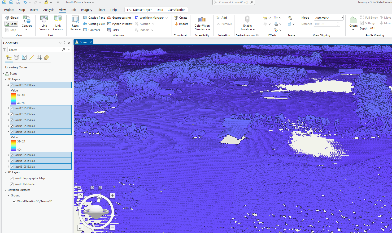
As with the Mesa County Colorado tiles, each North Dakota tile is distinct from the other. Expand the symbology under a couple of the .las files. Note, as with the Mesa County tiles, the symbology values for the color ramp vary because of the variation in values by tile (Figure 10.25). The next chapter explains how to manage this variation.

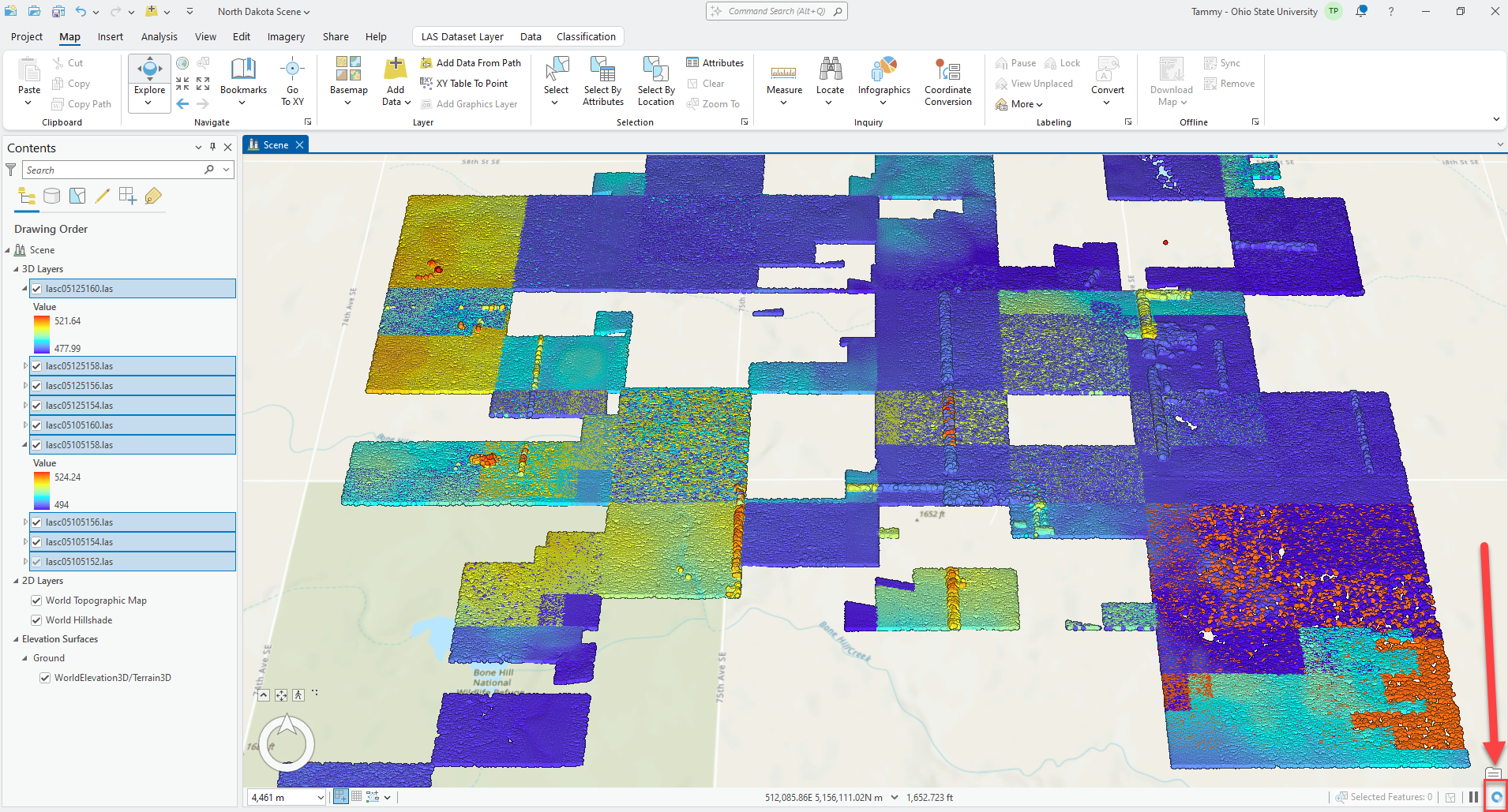
Use the same tools to navigate the scene with one exception that will be covered below. Watch the spinning circle in the lower right-hand corner while navigating and be sure that the points are completely populating (arrow pointing to the red box in Figure 10.26). Depending on point density, it may take longer to load the point cloud when zooming in.

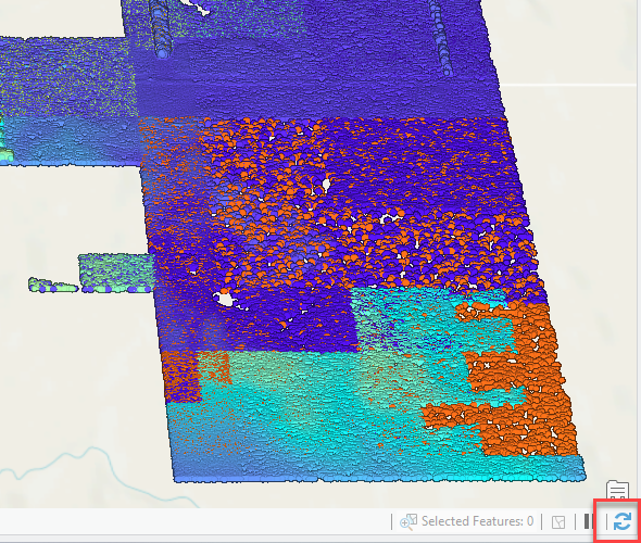
When ArcGIS Pro® finishes loading the point cloud, the icon changes to a refresh icon (re box, Figure 10.27).

Because the tiles are large files, this delay in loading the point cloud is ArcGIS Pro®’s way of managing large amounts of data. These settings can be adjusted and will be covered in a subsequent chapter.

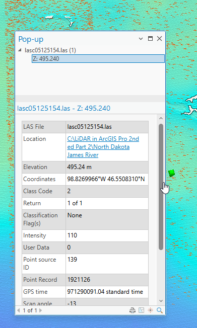
As in a Map template, clicking a point in the map viewer will identify attributes for a specific point (Figure 10.28).

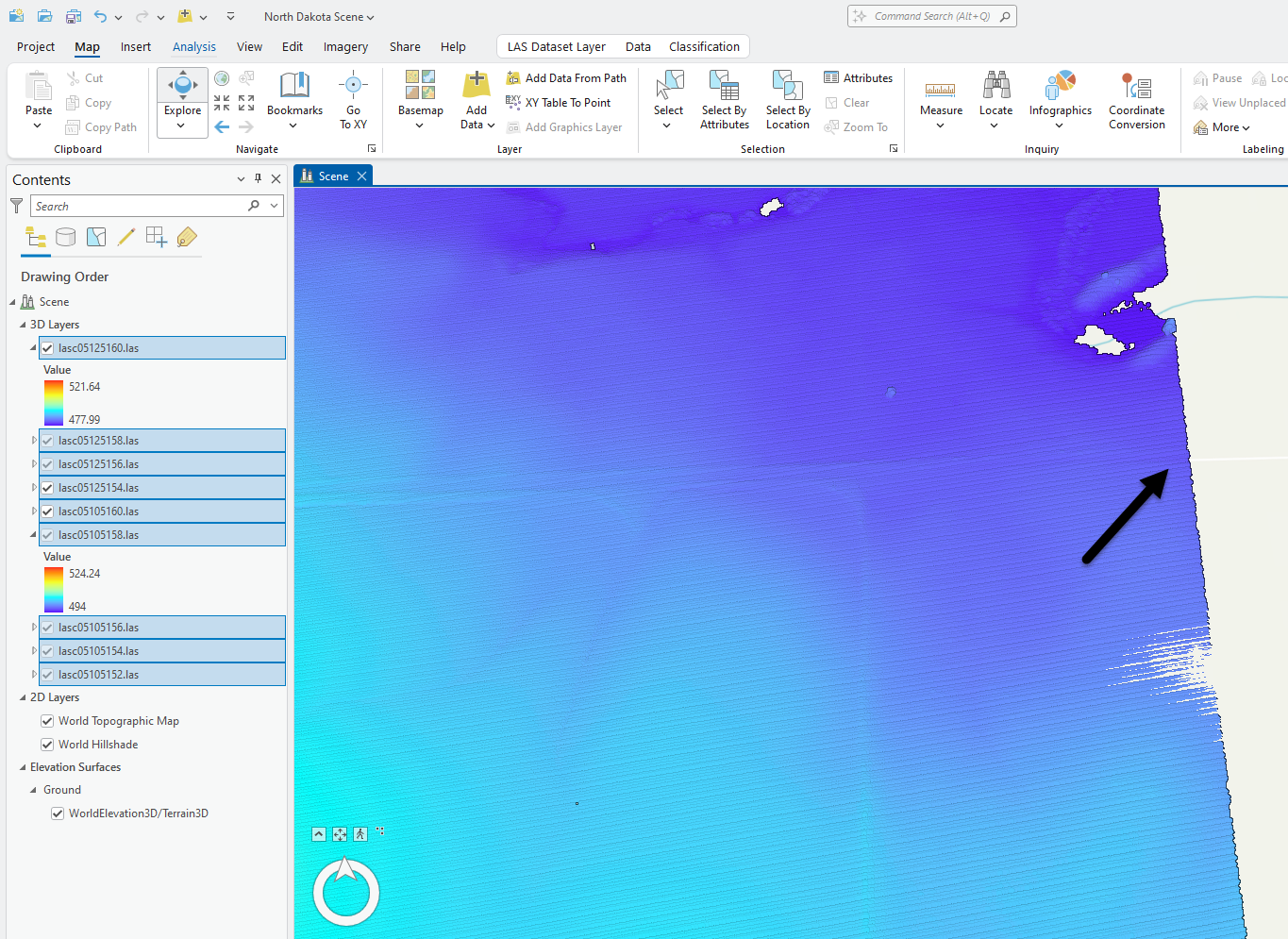
Zoom in to the area of the northeast corner of the southeast tile (Figure 10.29).

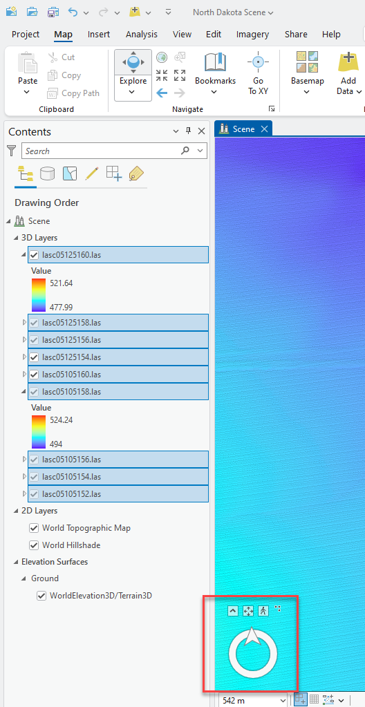
Because you are in a Scene, Navigator should be in the bottom left corner of the Scene(Figure 10.30).  If it is not showing, select View > Navigator as demonstrated above to activate it.

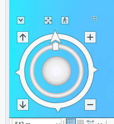
Expand Navigator. Navigator provides added functionality in the Local Scene Template (Figure 10.31).

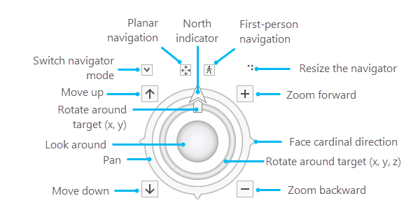
Additional options are now on the left side of Navigator—up and down arrows—that correspond to move up, move down (Figure 10.32).

Point to the east side of the outer ring, the east triangle turns blue (Figure 10.33).

Clicking on the blue triangle rotates the scene so East is at the top of the map viewer. Go ahead and experiment with the outer ring settings, then place it back so that North is at the top.

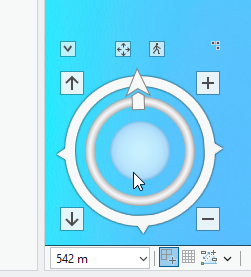
Navigator also now has an inner circle inside the inner ring (Figure 10.34)—this allows the map viewer to show the Scene from above or with an oblique view.  It also allows you to place a target on the map viewer.

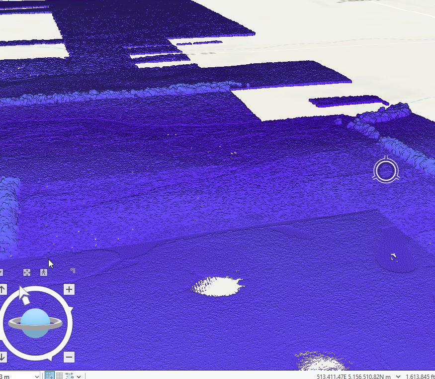
Point to a position in the Scene viewer, then depress the mouse wheel until the target is visible (Figure 10.35).

Hold down the mouse wheel, and when the ball inside the target displays (Figure 10.36), the scene can be tilted.  Move the mouse to practice tilting the scene. How it tilts depends on where the ball moves outside the target.

Don’t panic if it is not working. It takes some practice to accomplish this navigation skill.

When the scene tilts, the center circle and inner ring inside Navigator also tilts, providing an additional visual for map orientation.

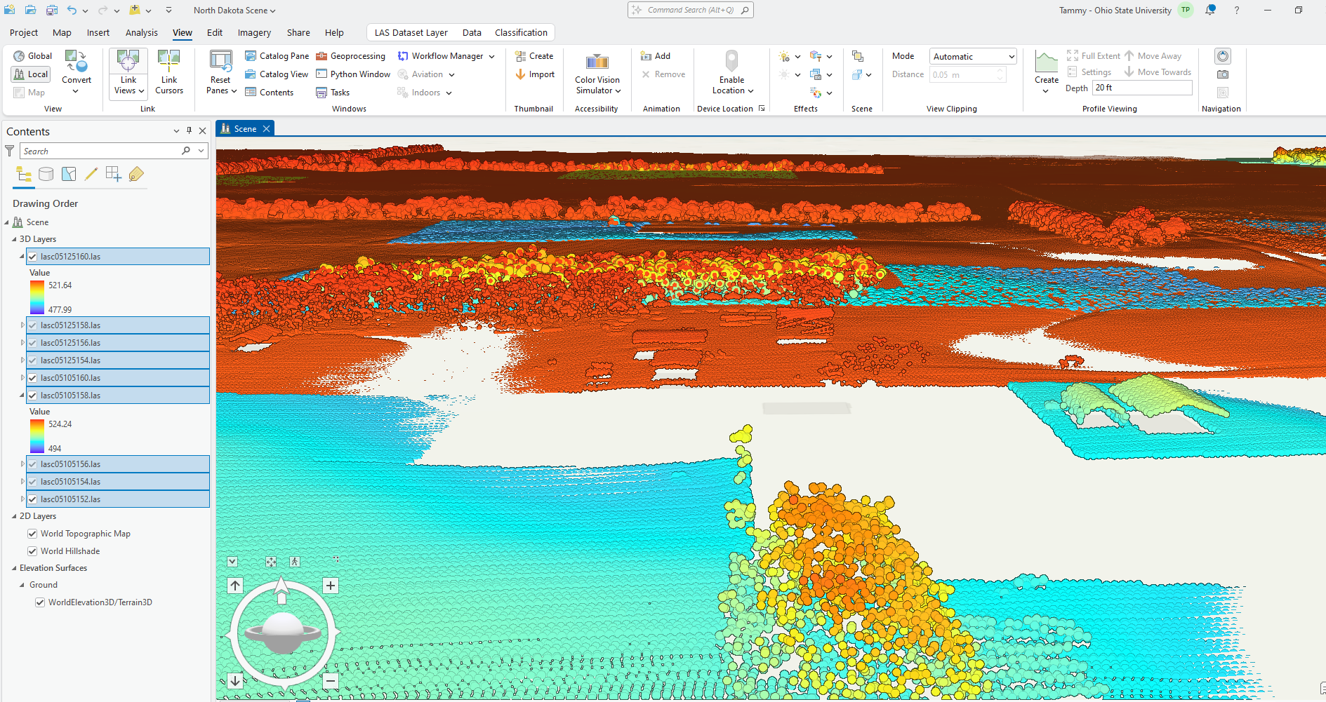
Features can now be identified in the point cloud—multiple buildings, silos, and trees.

Practice navigating and zooming over the point cloud (Figure 10.37).

Tilt can also occur by dragging the inner ring (not the center sphere) of the Navigator. Dragging the center sphere moves the target around the landscape (Figure 10.38).

Remember, when zooming in and out, the display must fill in the point cloud, so be patient.

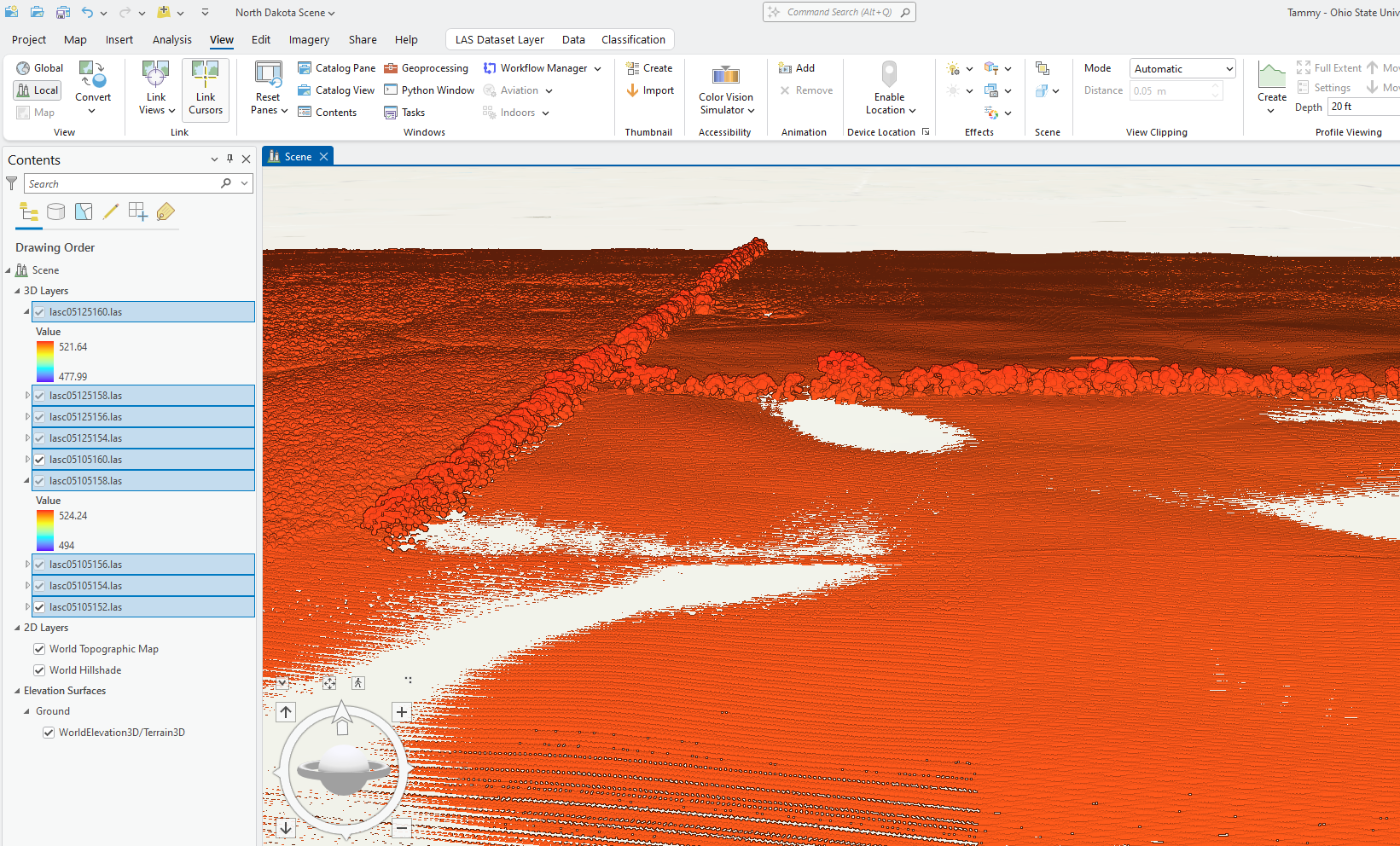
Find this location (Figure 10.39).

What is the linear feature in Figure 10.40? Tree-lined road, perhaps?

Display an absolute horizontal view, also called a profile view (Figure 10.41). Notice that the Navigator’s inner sphere is horizontal.

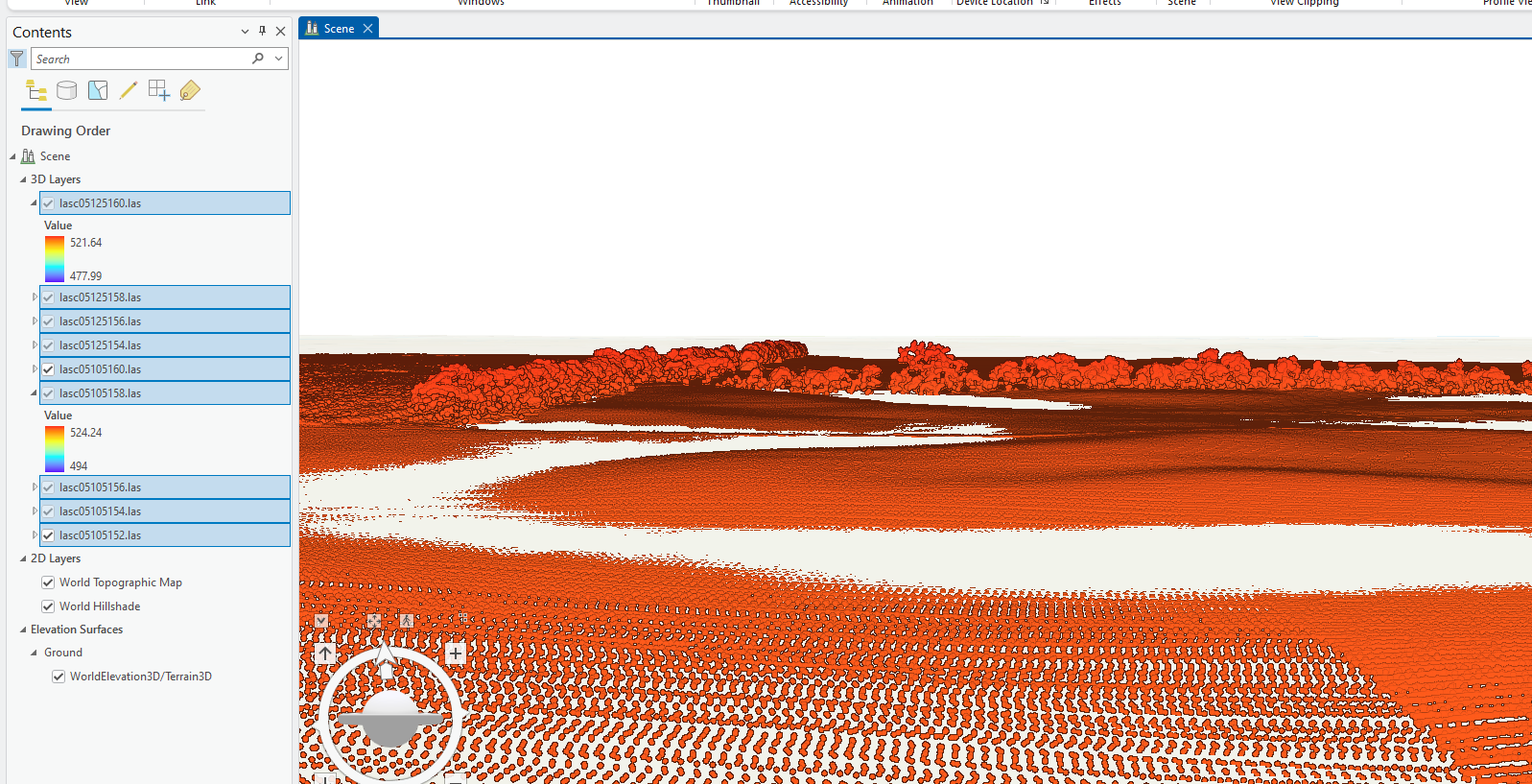
Navigating in 3D takes practice, so practice.

Finally, the navigation options can be changed by clicking on the Project tab on the ribbon (Figure 10.42). Click on Options (black box) and choose Navigation. These settings would strictly be personal preference and will not be reviewed here.

This concludes the introduction to lidar in ArcGIS Pro® and navigation. The next few chapters will introduce tools available under the LAS Dataset Properties section of ArcGIS Pro®. Chapter 13 provides instruction on creating one file from multiple downloaded tiles.