Chapter 16. Lidar Symbology

Prior chapters introduced lidar data, where to find lidar data on the internet, and how to download, unzip, load, and display the data in ArcGIS Pro® using a map template and a scene template. This chapter will introduce lidar symbology settings and options. Throughout this chapter, you will also use Google Earth® to help interpret terrain features. Reconnaissance-level interpretation of Google Earth® imagery can be helpful to augment your knowledge of landscape features, especially in unfamiliar areas. Using Google Earth® and other image services can help you identify objects on the ground. Aerial imagery is also served through ArcGIS Pro®.

Chapter 15. Lidar Display Settings demonstrated how to change settings to display a portion of the point cloud. This chapter illustrates symbology, including symbolization types and types of points, using the San Luis Valley data in a map scene. Lidar symbology in a map template is handled similarly but without 3D capabilities.

Open the San Luis Valley scene created in Chapter 13. Combining Tiles into One .lasd Dataset (Figure 16.1).

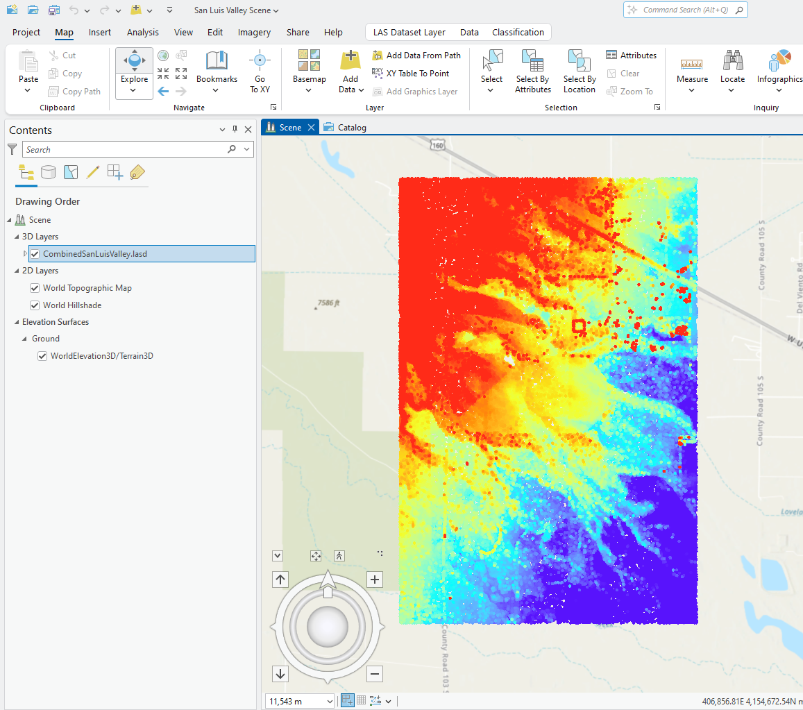
Unlike vector data, Lidar data does not have an attribute table. But each lidar point can have different characteristics. ArcGIS Pro® uses elevation as the default symbology. In Figure 16.1, the symbology is provided as a color ramp, using elevation as the value (other values can be used for display and will be covered later in this chapter). But what is the unit of measurement?

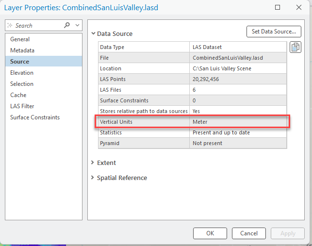
The unit of measurement can be located by right-clicking on the file name and going to Properties >Source > Vertical Units. The unit is Meter (Figure 16.2). 

Elevation is typically thought of as land height above mean sea level. But all lidar data points have elevation values, even if the point represents vegetation, debris floating in water, a bird or a building’s roof. It is important to understand that the elevation value assigned to a vegetation point is its height above mean sea level. To obtain the actual height of vegetation or a building roof (from ground level) using lidar data, it will be important to know the elevation of the bare earth under the building (or associated with the base of the building).

Let’s clarify some issues that arise before discussing symbology.

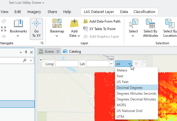
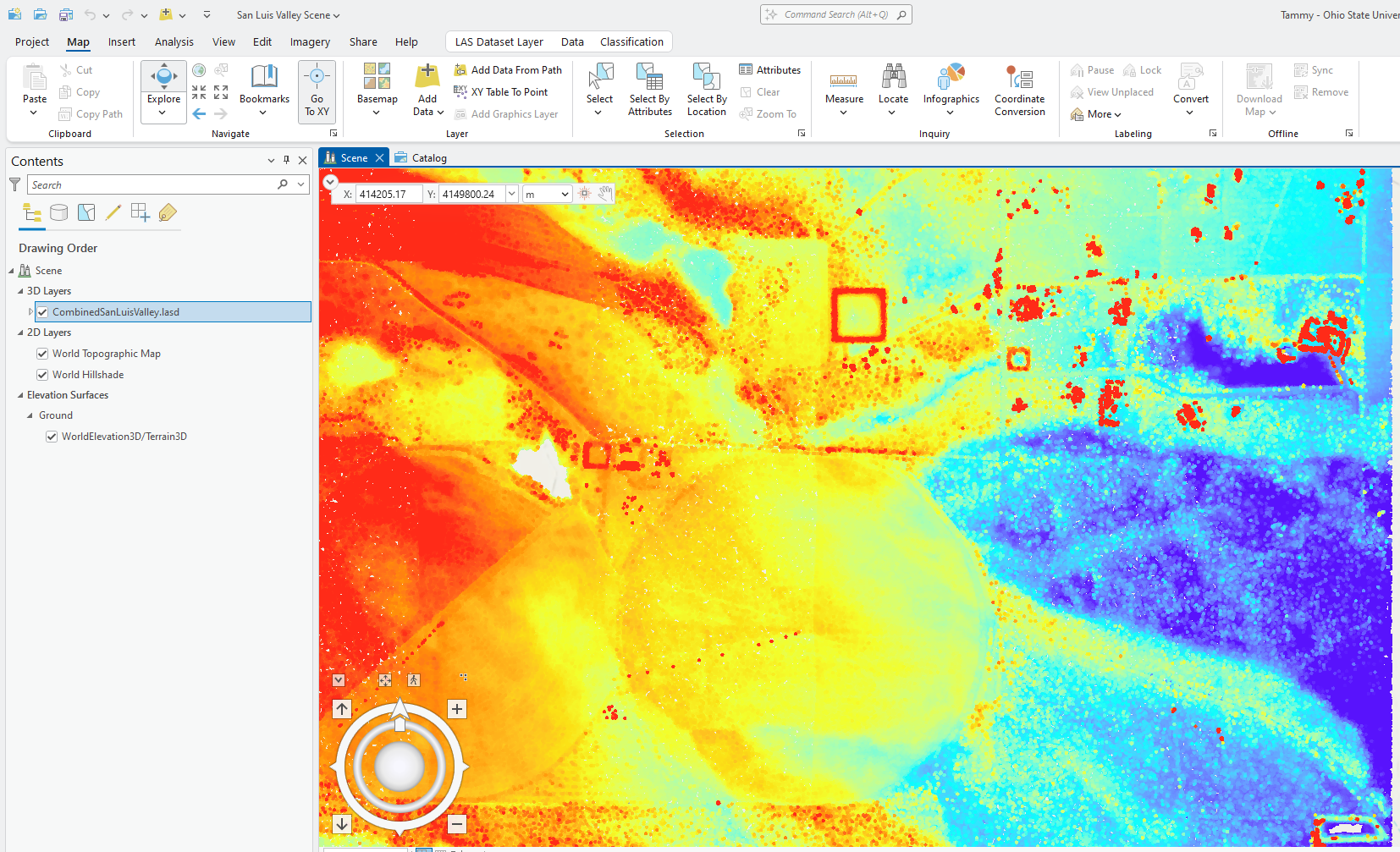
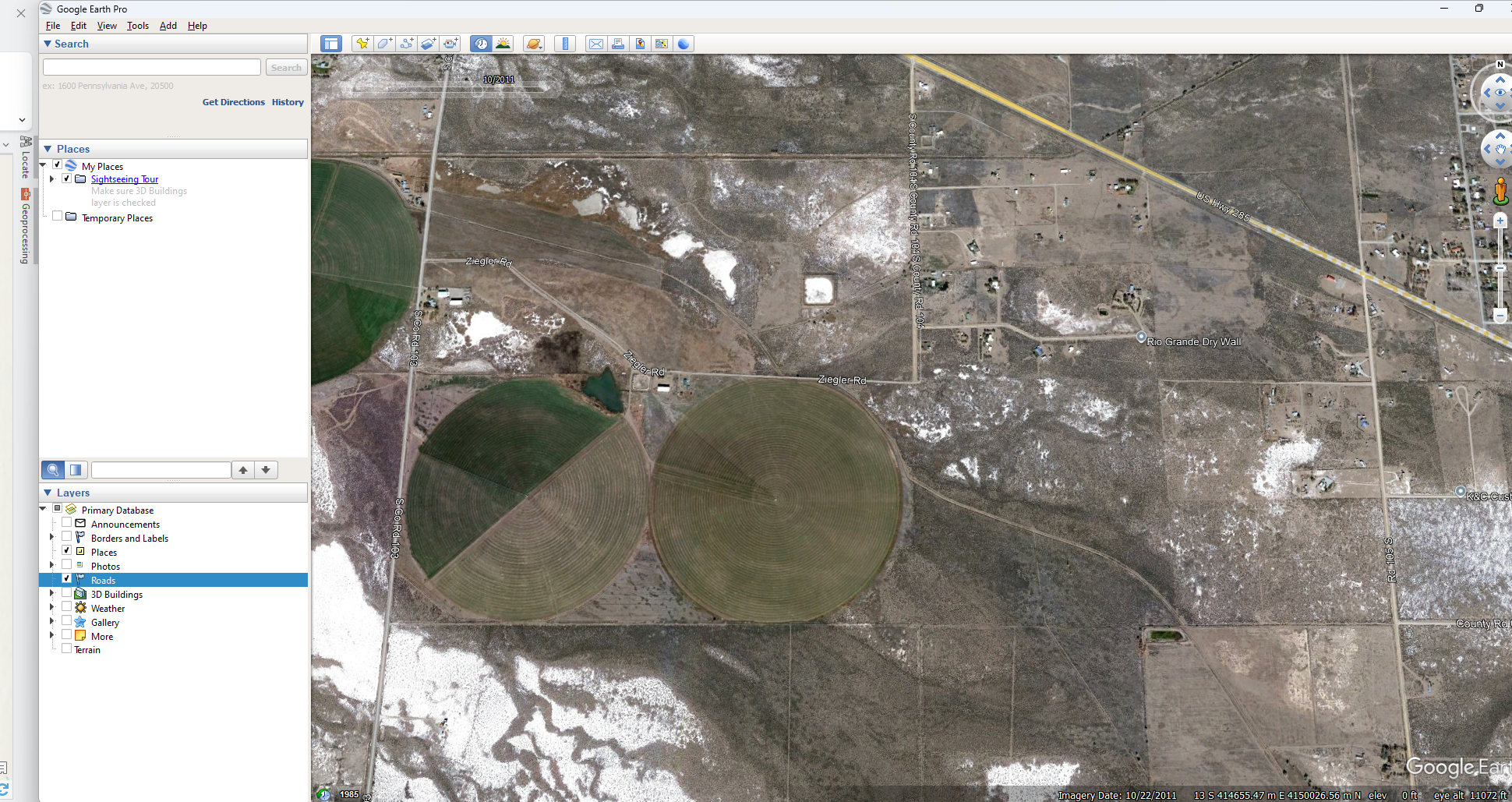
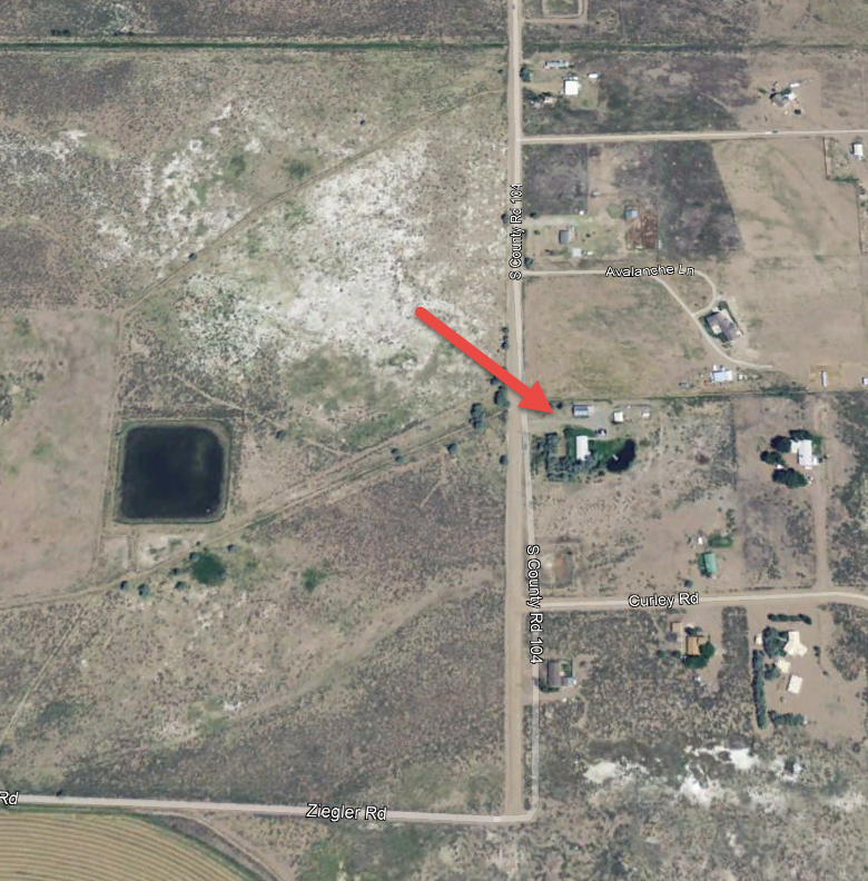
Using the Go to XY tool (Figure 16.3), zoom in to the location shown in Figure 16.4. Do you recognize any features? See the large circular irrigated crop field, also known as center pivot irrigation system or sometimes referred to as a crop circle? It is due south of the square feature.

The values below the map display (at the bottom of the viewer, Figure 16.4) represent the UTM coordinate values and elevation values for the center of the center pivot irrigation system, also known as a crop circle. Note that in this example, UTM values are expressed in meters, and elevation values are expressed in feet.

Open Google Earth Pro®. Enter the coordinate values in the Search tool to navigate to this exact location in Google Earth® (Figure 16.5).

Imagery can be added as a basemap in ArcGIS Pro®. However, in most instances, the acquisition date of the imagery is not known. Using Google Earth Pro® as an additional source of reference imagery provides additional imagery dates, and potentially additional information about terrain features. Google Earth Pro® also provides the option to access historically archived imagery. This can be useful to examine trends over time, and to match lidar acquisition dates with imagery acquisition dates as closely as possible. Additionally, 2D imagery displayed in a 3D scene often creates an overlay mismatch (as demonstrated below).

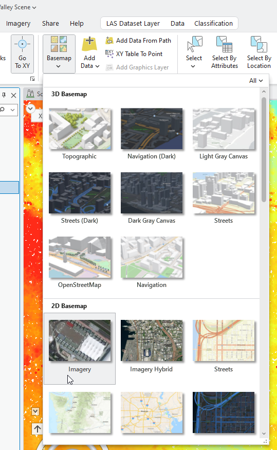
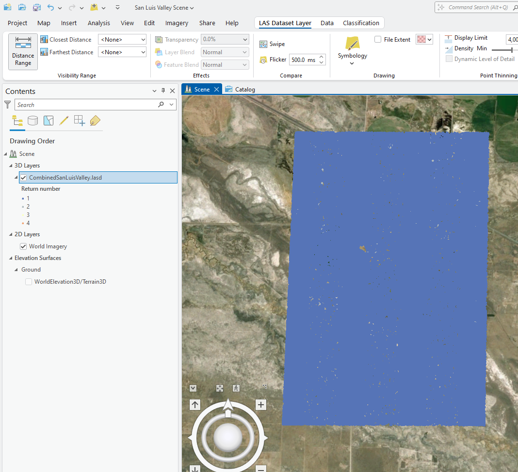
In Contents, turn off the Topographic, World Hillshade and WorldElevation layers. Go to the Map tab on the ribbon, click on Basemap and select Imagery  from the 2D Basemap group(Figure 16.6). The imagery is not viewed in the map viewer because it is beneath the lidar data. However, the World Imagery layer is listed in the Contents pane.

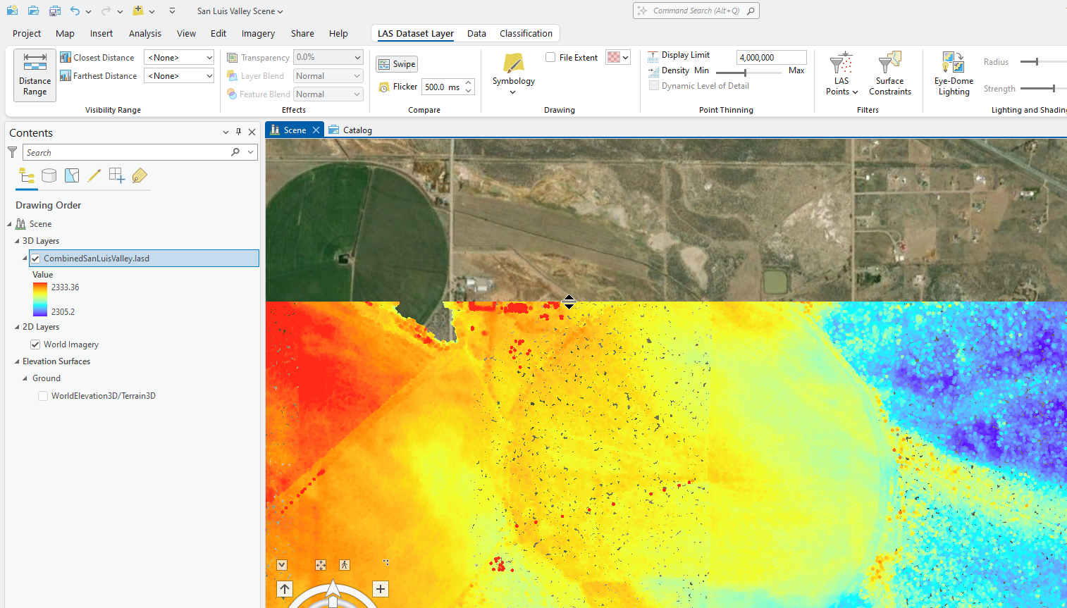
Now use the Swipe or Flicker tool to see the image under the lidar point cloud (Figure 16.7), an exact overlay does not occur. There are several reasons for this. The first reason is that there is a projection overlay issue. The layers are associated with two different projections—one for the lidar data and one for the basemap imagery. Second, 3D data (lidar) is overlaid on a 2D map (imagery). And third, the lidar data are positioned at a vertical distance of 16,698 feet above the basemap—see the status bar in ArcGIS Pro, it is not showing in Figure 16.7.

So be very cautious when using imagery within ArcGIS Pro® as a basemap layer in a 3D scene.

Now, back to the original message that the elevation value symbolized in contents is also the value of height for other features.

Pan east of the large square to the small square and the house just south of the small square (Figures 16.8 and 16.9). Focus on the roofline of the house and trees.

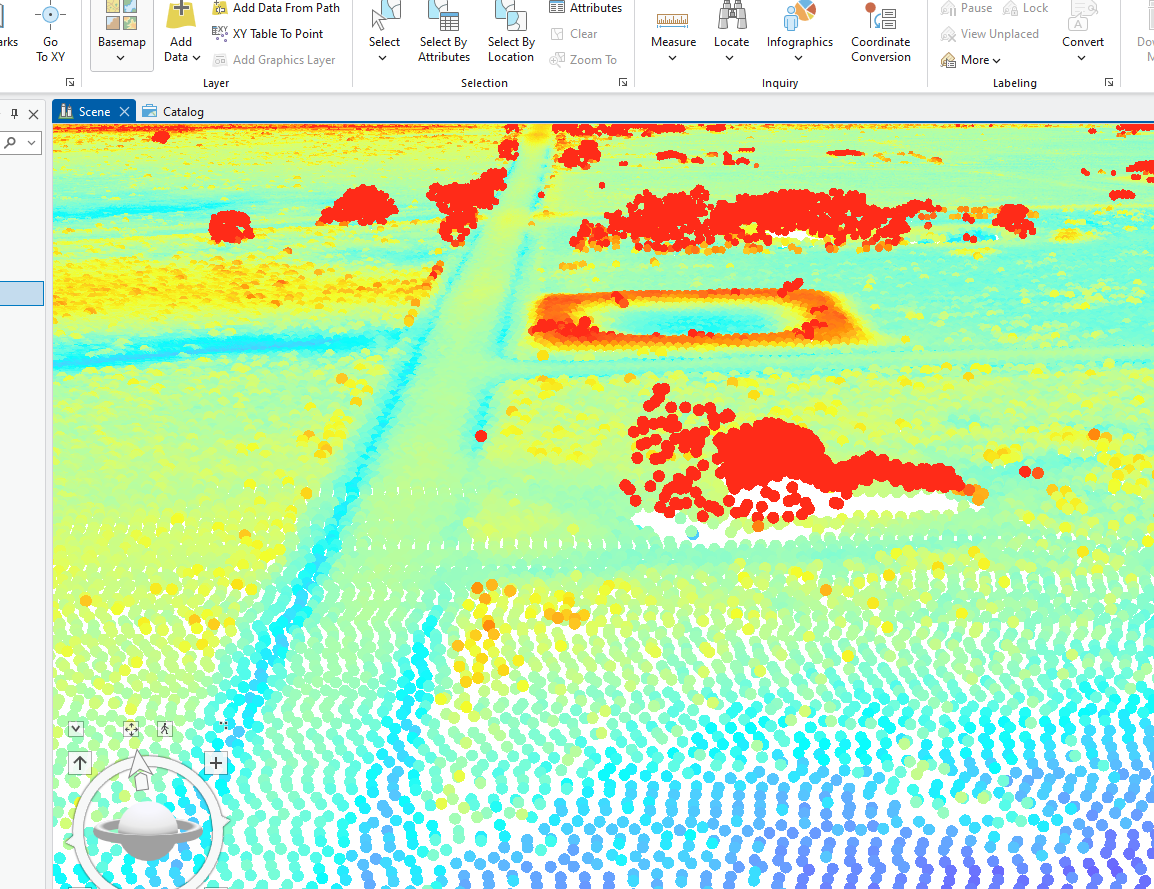
Use 3D navigation demonstrated in Chapter 5. Vector Symbology to view a profile of the house and trees (Figure 16.10).

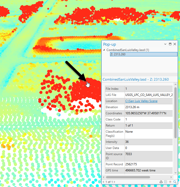
Now identify one point on the peak of the roof of the house (Figure 16.11). The elevation reading is 2,313.26 meters. Does this mean that the structure is 2,313 meters high, or 2,313 meters above sea level?

Now zoom back out and pick a point on the far west side of the point cloud. Can you zoom to the point identified in Figure 16.12? It is a bare earth elevation point (coordinates are found in the Pop-up dialog, then use Go To under the Map tab). The elevation for this point (a ground-based point) is 2,310.73 meters.

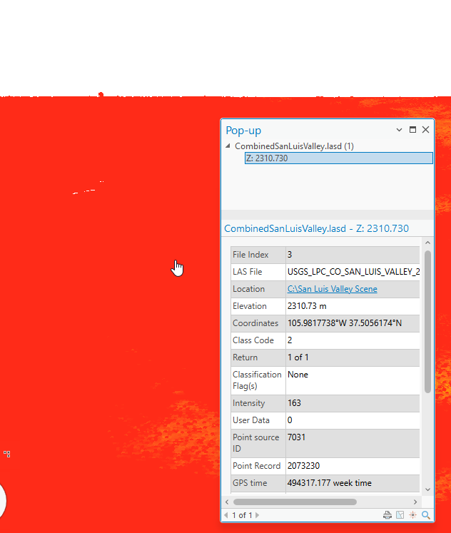
Why go through this example and review? Remember, the discussion started with using elevation as the symbology, but when using lidar data, you need to remember that the elevation values do not necessarily reflect the elevation of the ground. Lidar data provide the height of all measured data points, which could include treetops, the tops of buildings, the tops of cars, etc.

Now, let’s change the symbology. Leave all points displayed (except where noted below) as it will help with navigating to different areas of this region by showing distinctive features like trees and roofs.

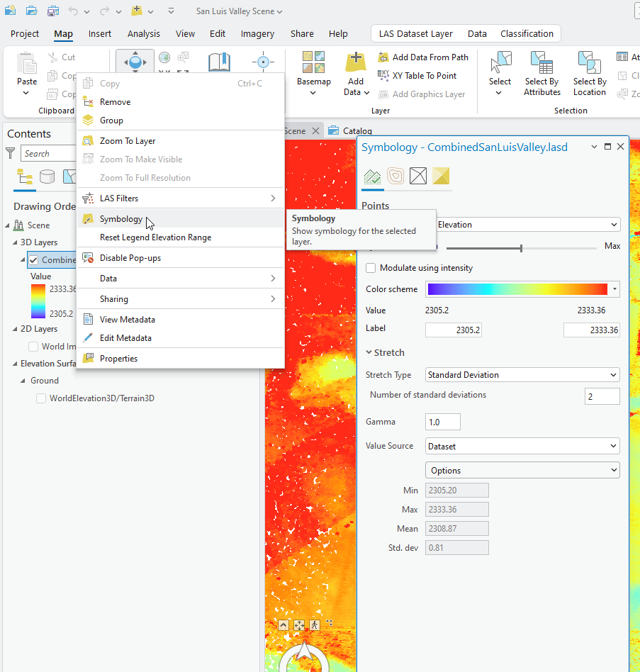
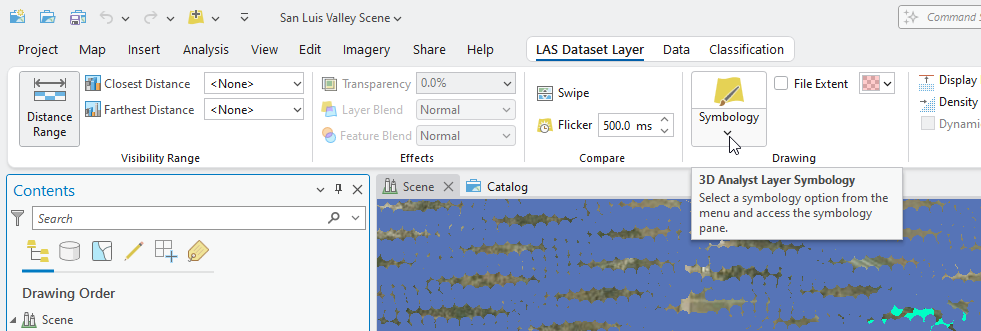
Right-click the layer name and choose Symbology (Figure 16.13). The symbology dialog box opens.

Change the point type by clicking the down arrow at the end of Draw Using (Figure 16.14).

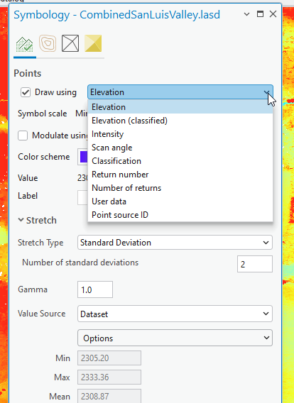
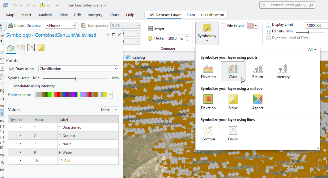
Change it to Classification (Figure 16.15). Remember from Chapter 5. Vector Symbology that in ArcGIS Pro®, symbology automatically changes.

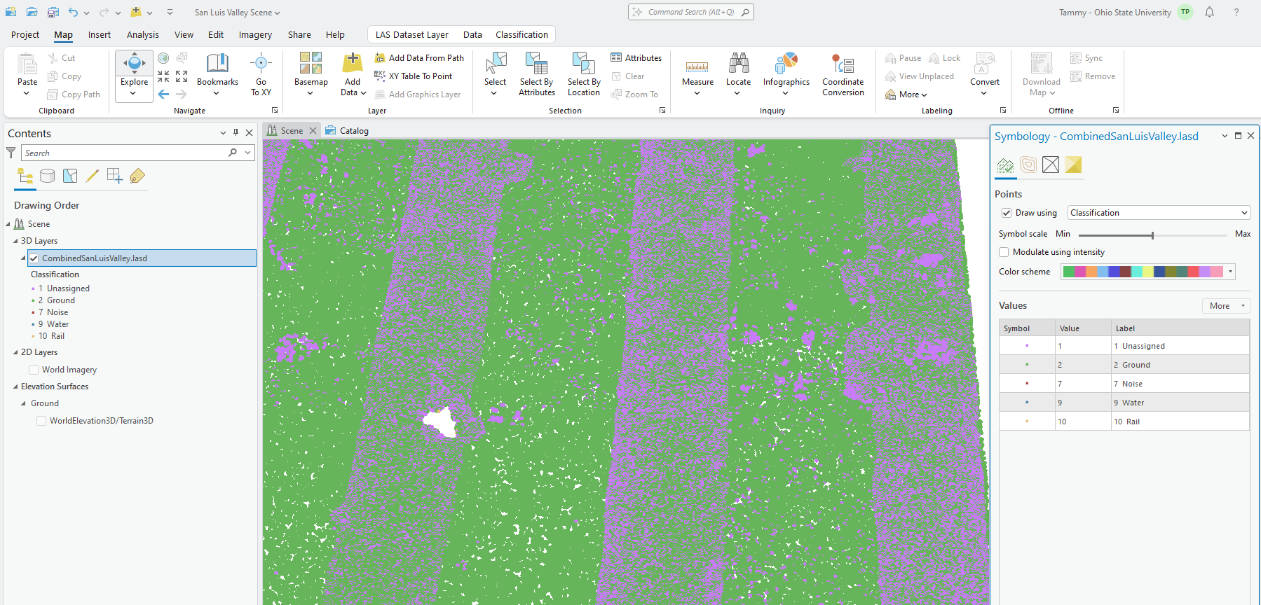
ArcGIS Pro® assigns a color scheme, but this can also be changed by clicking on the down arrow at the end of the Color scheme ramp.

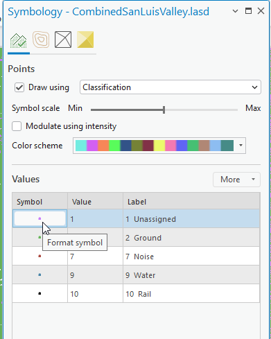
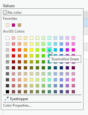
Because the number of classification symbols is limited for this scene, only 5 classification symbols are used: symbols associated with ground, noise, water, rail and unassigned. The color variation is minimal. A single symbol can also be changed. Click on an individual point symbol under Classification (Figure 16.16) and the points symbology dialog box appears (Figure 16.17). You can then choose a color desired for each individual symbol classification.

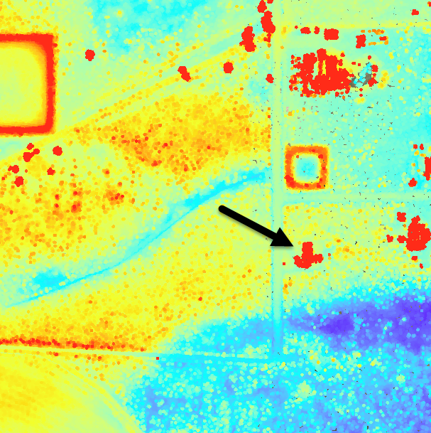
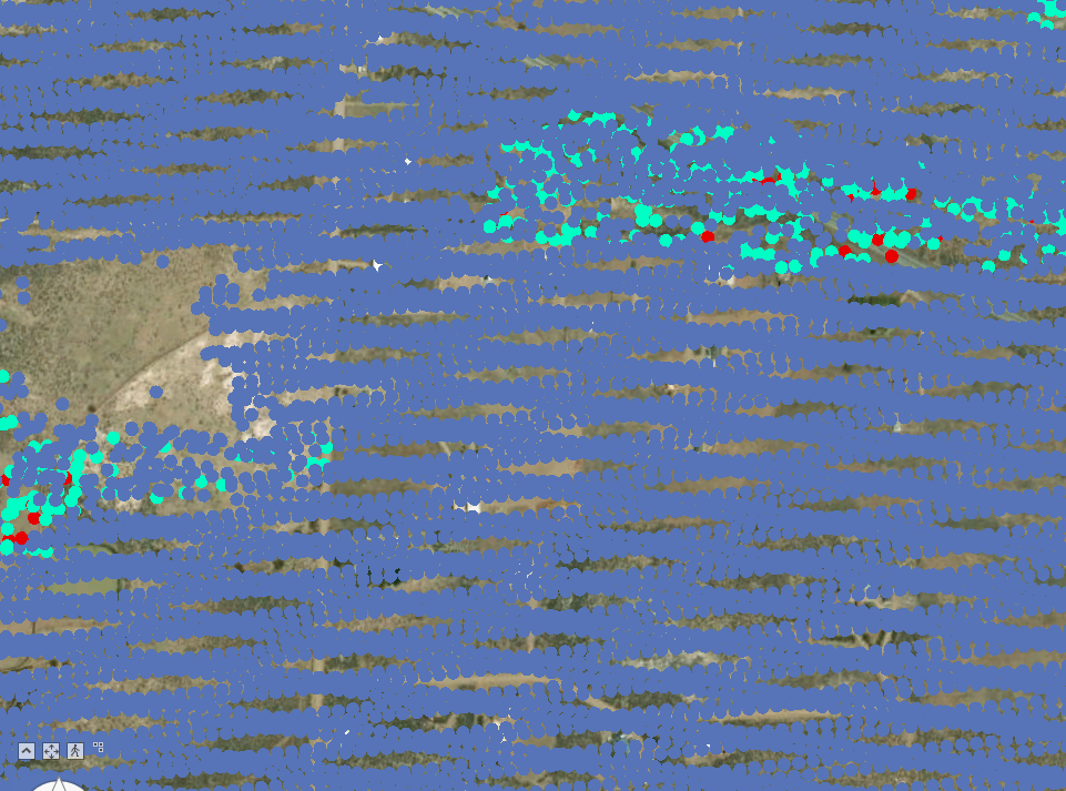
Although there are five classes listed, most of the point cloud is either associated with ground data returns or unassigned data returns, and so the image only appears to be associated with two colors. To see more classified data, zoom in to the empty area in the point cloud (Figure 16.18). Do you know why most of the point cloud is missing in this area of the image?

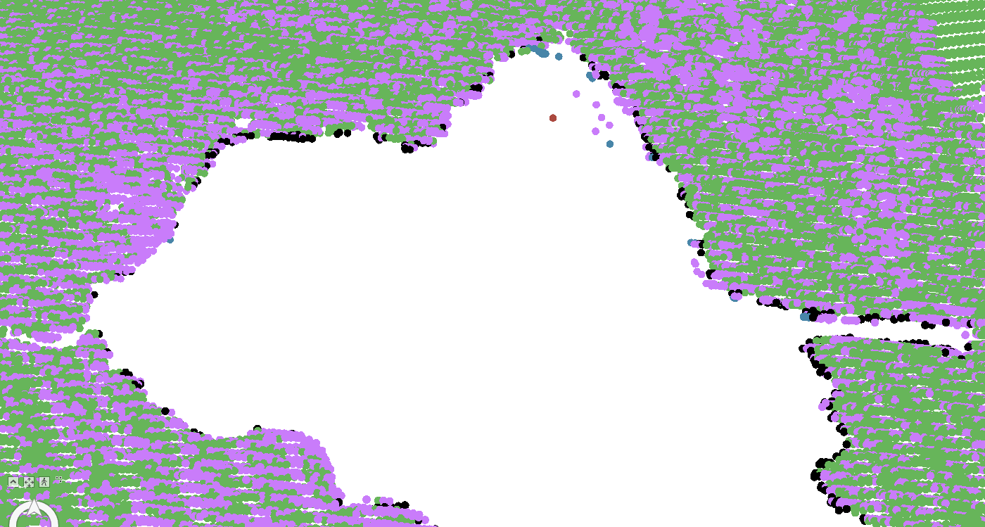
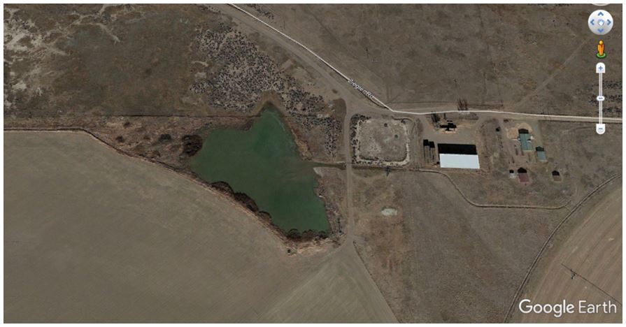
It is a water body (Figure 16.19 is from Google Earth®). Keep in mind that water absorbs lidar pulses, so these lidar points will not reflect back to the sensor when the water is deep, clear or calm. As seen in Figure 16.17, the edges of the pond include either vegetation or sediment laden water. The lidar returns from these edge areas may, therefore, reflect data, and will be associated with varied classifications in the point cloud (as seen in Figure 16.18).

Now, change the Symbology to Return Number. While this dataset had up to 4 returns, it appears from the resultant display that the returns were almost all first returns (Figure 16.20.).

Change the individual colors so they are more distinctive and then zoom in to an area (Figure 16.21). At least three different lidar data returns are now displayed—1st returns, 2nd returns, and 3rd returns.

Recall that only a portion of the point cloud is being displayed so it may be necessary to zoom in to get a better idea of the data spread over the returns. Why would an area include only first returns? It could be a region of all bare earth or entirely impervious surfaces—a relatively flat terrain with no vegetation present.

Symbology can also be changed under LAS Dataset Layer > Appearance > Symbology (Figure 16.22).

Clicking the down arrow under Symbology provides more options (Figure 16.21).

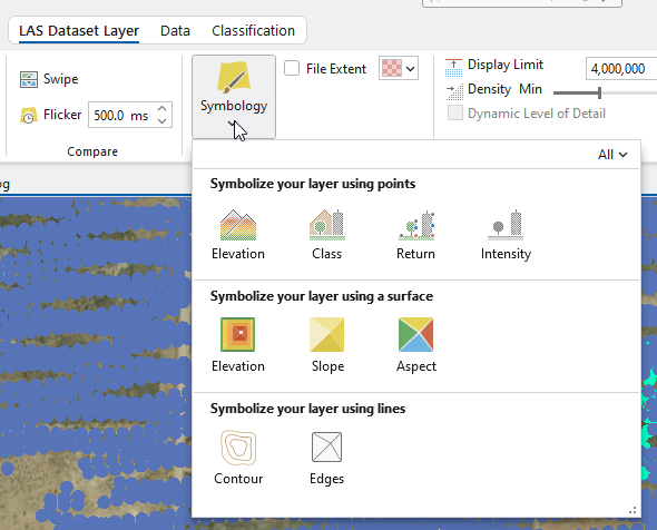
From the first row—Symbolize your layer using points —the same dialog opens as when right-clicking the layer name and choosing Symbology (Figure 16.24).

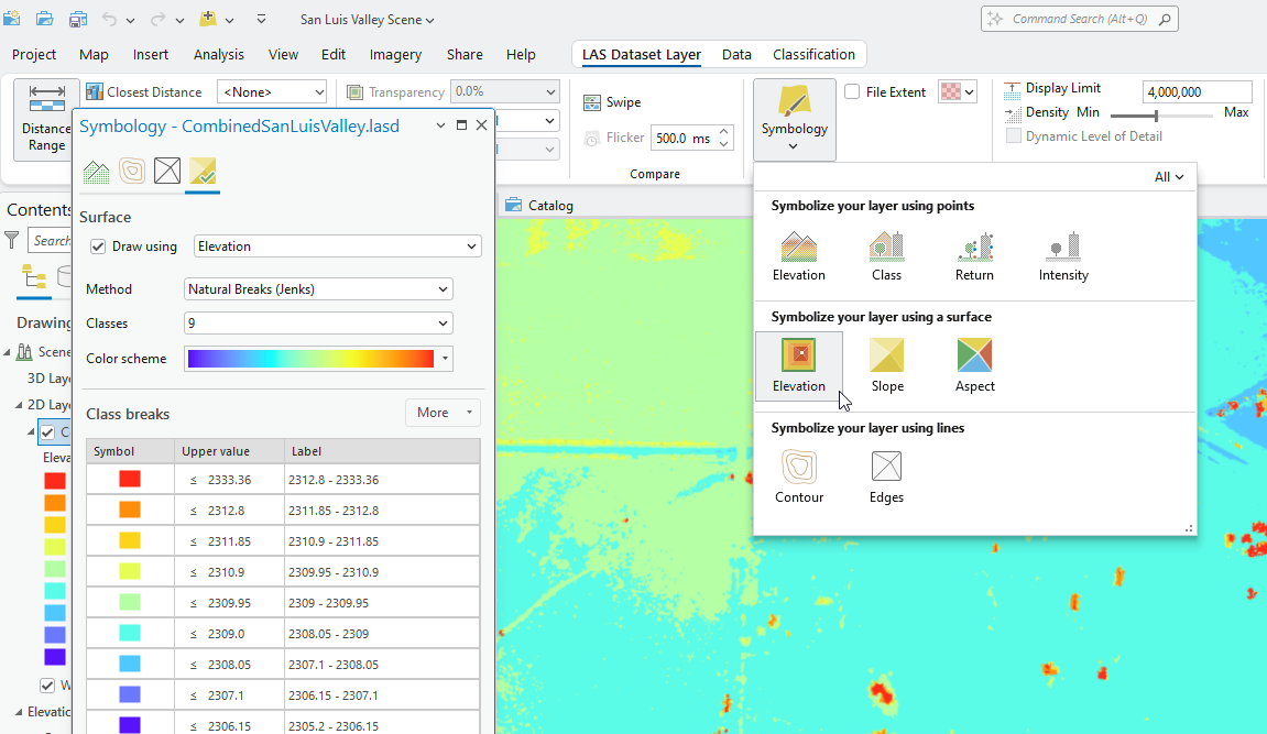
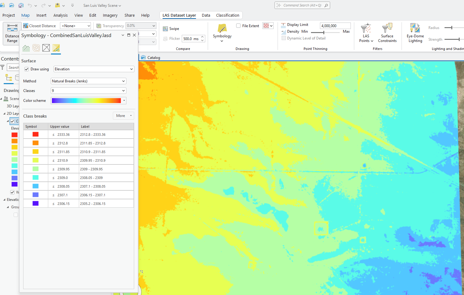
Choosing an icon from the second row—Symbolize your layer using a surface—classifies the elevations into nine ranges of values (classes) (Figure 16.25). The number of classes can be changed, under Classes.

Now change the display to Ground points only (see Chapter 15. Lidar Display Settings if a refresher is needed). Do you see the difference between Figure 16.25 using all points and Figure 16.26 using ground points only? The roof lines and vegetation are missing in Figure 16.26. This is because we have selected to display only the lidar data returns classified as ground.

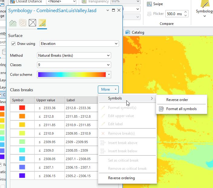
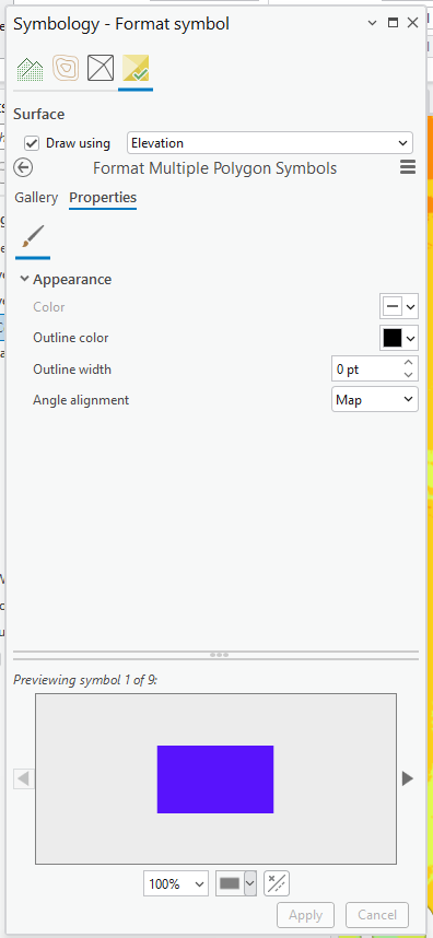
Choose the More down arrow to the right of Class Breaks, point to Symbols and choose Format all symbols (Figure 16.27).

A new dialog opens, Symbology – Format symbol, with two tabs—Gallery and Properties. Gallery allows a choice of symbols for each of the classified polygons (Figure 16.28). Feel free to explore these before proceeding.

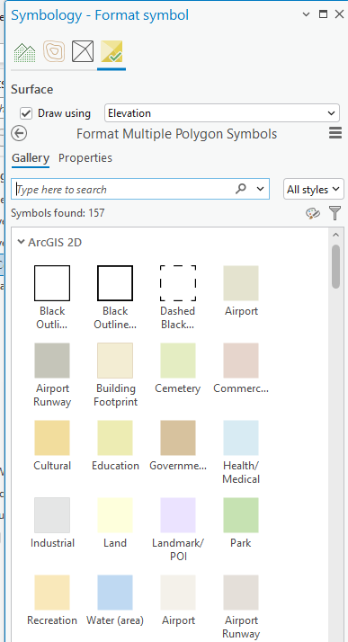
Properties allows additional symbolization, including adding an outline around each point (Figure 16.27). This chapter does not cover every option but feel free to explore. Please note that symbology options are display only so the actual dataset is not changed.  Close the dialog box when you have finished exploring.

Go back to Symbology > Symbolize your layer using a surface > Slope. Be sure to use ground points only (Figure 16.30). With slope, the number of classes can also be changed.

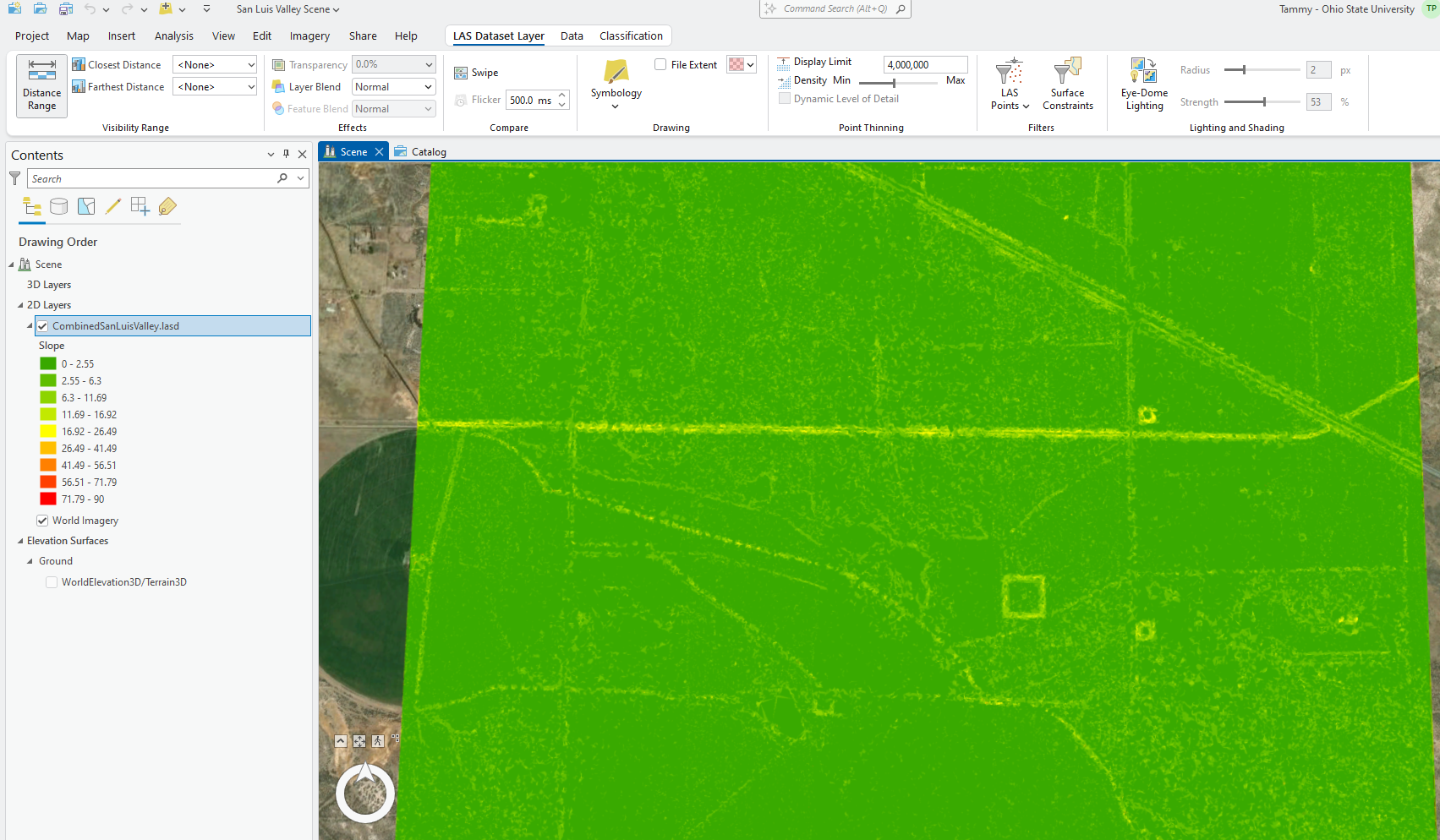
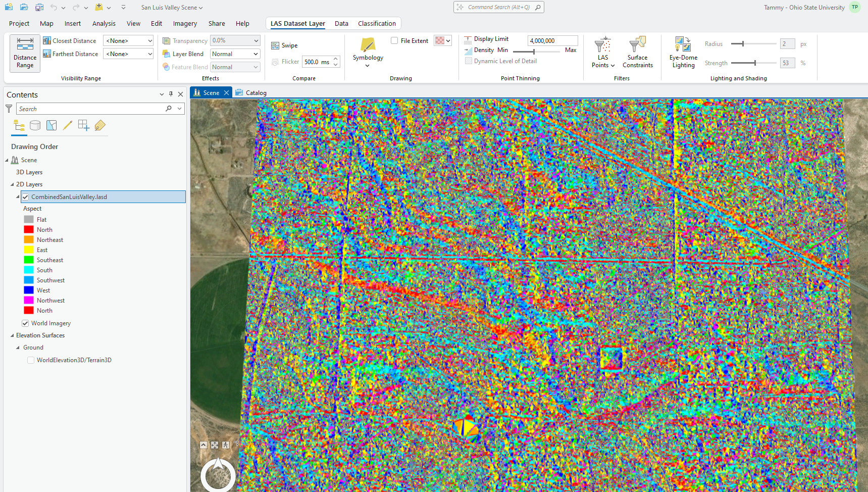
Figure 16.31 displays Aspect (with ground points only).

This concludes this chapter introducing symbology. The tools demonstrated in this chapter are for display purposes only. These options do not create an elevation file, a slope file or an aspect file so these displays cannot be used in any type of analysis.

Subsequent chapters (18 through 21) will demonstrate how to classify lidar points. Classification of all points must be completed before creating datasets that can be used in analyses, such as a digital elevation model, a slope dataset and an aspect dataset.