If you knew the length of someone’s pinky (smallest finger), do you think you could predict that person’s height? Imagine collecting data on this and constructing a scatter plot of the points on graph paper. Then draw a line that appears to “fit” the data. For your line, pick two convenient points and use them to find the slope of the line. Find the y-intercept of the line by extending your line so it crosses the y-axis. Using the slopes and the y-intercepts, write your equation of “best fit.” According to your equation, what is the predicted height for a pinky length of 2.5 inches? You have just started the process of linear regression.

Linear Regression

Data rarely perfectly fit a straight line, but we can be satisfied with rough predictions. Typically, if a dataset has a scatter plot that appears to “fit” a straight line called a line of best fit or least-squares line. This process of fitting the best-fit line is called linear regression.

The equation of the regression line is ŷ =a+bx.

The ŷ is read “y hat” and is the estimated value of y obtained using the regression line. It may or may not be equal to values of y observed from the data.

The sample means of the x values and the y values are and , respectively. The best fit line always passes through the point (, ).

The slope, b, can be written as , where s_y is the standard deviation of the y values and s_x is the standard deviation of the x values. Note that the slope is directly calculated using r, the correlation coefficient, discussed in previous sections.

The y-intercept, a, can then be calculated by using the slope, and means of x and y.

Example

Recall our previous example:

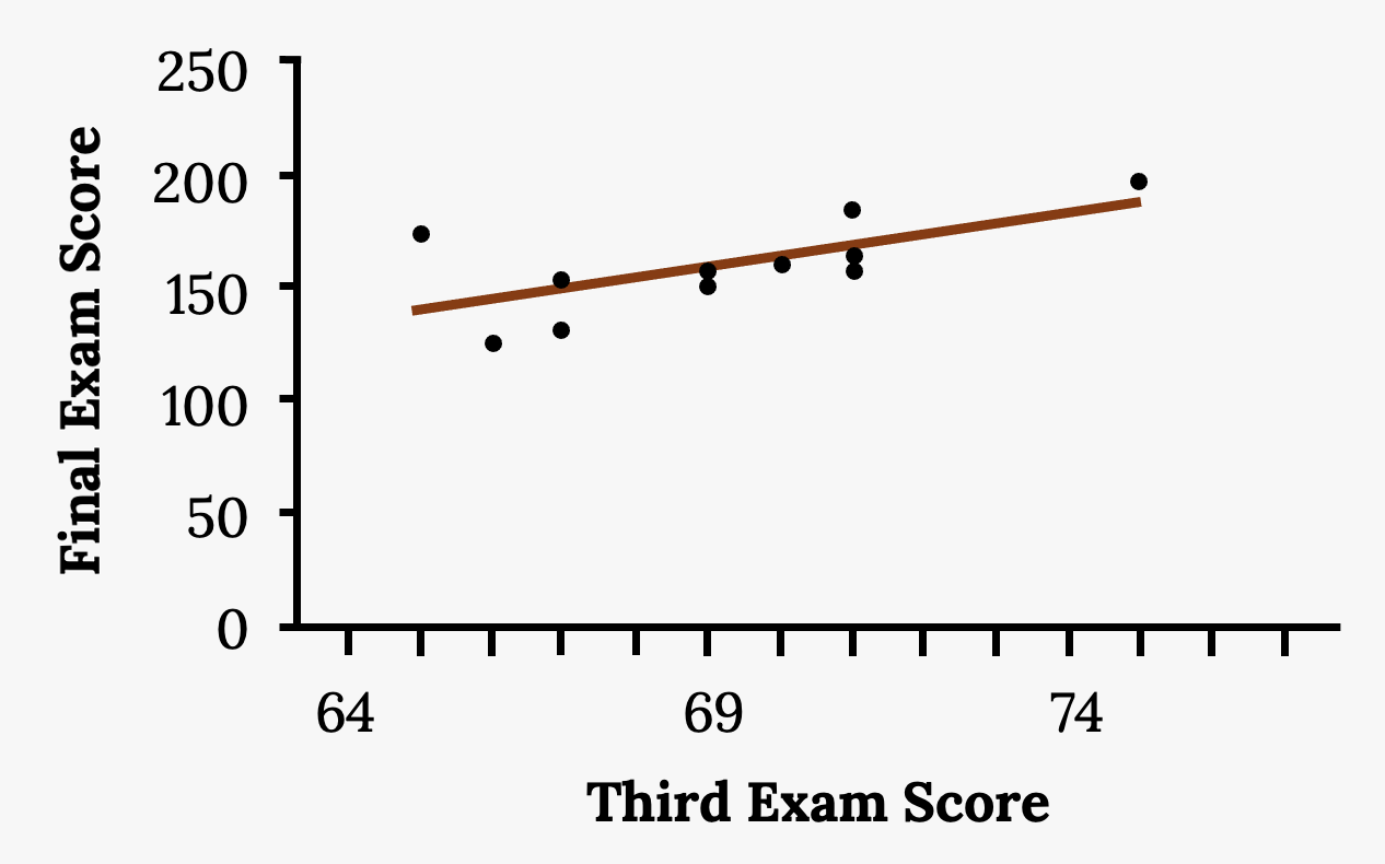
A random sample of 11 statistics students produced the following data, where x is the third exam score out of 80, and y is the final exam score out of 200. Can you predict the final exam score of a random student if you know the third exam score?

Third exam score	Final exam score
65	175
67	133
71	185
71	163
66	126
75	198
67	153
70	163
71	159
69	151
69	159

Figure 3.16: Third and final exam scores data

 

Solution

We have found:

• An apparent linear relationship in the scatterplot
• The correlation coefficient is r = 0.6631
• The coefficient of determination is r² = 0.66312 = 0.4397

The third exam score, x, is the independent variable and the final exam score, y, is the dependent variable. We will plot a regression line that best “fits” the data. If you were to fit a line “by eye,” you may draw different lines. We most often use what is called a least-squares regression line to obtain the best fit line. The idea behind finding the best-fit line is based on the assumption that the data are scattered about a straight line. The criteria for the best fit line is that the vertical distance of each point to the line is minimized, that is, made as small as possible. This best fit line is called the least-squares regression line.

Consider the following diagram. Each point of data is of the form (x, y), and each point of the line of best fit using least-squares linear regression has the form (x, ŷ).

 

 

Solution

The line of best fit is: ŷ = –173.51 + 4.83x

Your Turn!

SCUBA divers have maximum dive times they cannot exceed when going to different depths. The data in the figure below show different depths’ maximum dive times in minutes. Use your calculator to find the least-squares regression line and predict the maximum dive time for 110 feet.

Depth (in feet)	Maximum dive time (in minutes)
50	80
60	55
70	45
80	35
90	25
100	22

Figure 3.18: SCUBA diver stats

Understanding Slope

The slope of the line, b, describes how changes in the variables are related. It is important to interpret the slope of the line in the context of the situation represented by the data. You should be able to write a sentence interpreting the slope in plain English.

Interpretation: The slope of the best-fit line tells us how the dependent variable (y) changes for every one unit increase in the independent (x) variable on average.

Understanding the y-Intercept

The y-intercept of the line, a, can tell us what we would predict the value of y to be when x is 0. This may make sense in some cases, but in many, it may not make sense for x to be equal to 0, therefore the y-intercept may not be useful.

Prediction

The next and most useful step in regression is to actually use that equation to predict future values of y.

Recall our example in which we examined the scatter plot and found the correlation coefficient and coefficient of determination. We found the equation of the best-fit line for the final exam grade as a function of the grade on the third exam. We can now use the least-squares regression line for prediction.

Figure References

Figure 3.17: Kindred Grey (2020). Line of best fit. CC BY-SA 4.0. Adaptation of Figure 12.11 from OpenStax Introductory Statistics (2013) (CC BY 4.0). Retrieved from https://openstax.org/books/introductory-statistics/pages/12-3-the-regression-equation