13 Deserts and Glaciers
Learning Objectives
By the end of this chapter, students should be able to:
- Explain the defining characteristics of a desert, and distinguish among the broad categories of deserts.
- Explain how geographic features, latitude, atmospheric circulation, and Coriolis effect influence where deserts are located.
- List the primary desert weathering and erosion processes and resulting landforms.
- Identify desert landforms, and explain how they are formed by erosion and deposition.
- Describe the main types of sand dunes and the conditions that form them.
- Differentiate the different types of glaciers, and contrast them with sea icebergs.
- Describe how glaciers form, move, and create landforms.
- Describe glacial budget; describe the zones of accumulation, equilibrium, and melting.
- Describe the history and causes of past glaciations and their relationship to climate, sea-level changes, and isostatic rebound.
At first glance, deserts and glaciers may seem like opposites—one conjures images of endless heat and aridity, while the other evokes thoughts of frozen, icy expanses. However, both deserts and glaciers are part of a larger conversation about extreme environments shaped by similar geological forces. These landscapes are defined by scarcity, either of water or warmth, and both are profoundly influenced by processes of erosion, deposition, and weathering.
Deserts, which cover about one-third of the Earth’s land surface, are characterized by their dry conditions, where evaporation exceeds precipitation. Although glaciers are composed of frozen water, they can be considered “frozen deserts” because they too exist in regions where precipitation is low, albeit in solid form. In both environments, the absence or freezing of water leads to unique landforms and geologic features. Understanding these landscapes not only enriches our appreciation of the diversity of Earth’s environments but also highlights their vulnerability to climate change.
This chapter is divided into two parts; the first half explores the characteristics, formation, and geological processes of deserts, while the second half delves into the features and dynamics of glaciers.
13.1 The Origin of Deserts
Approximately 30% of the Earth’s terrestrial surface consists of deserts, which are defined as locations of low precipitation. While temperature extremes are often associated with deserts, they do not define them. Deserts exhibit extreme temperatures because of the lack of moisture in the atmosphere, including low humidity and scarce cloud cover. Without cloud cover, the Earth’s surface absorbs more of the Sun’s energy during the day and emits more heat at night.
Deserts are not randomly located on the Earth’s surface. Many deserts are located at latitudes between 15° and 30° in both hemispheres and at both the North and South Poles, created by prevailing wind circulation in the atmosphere. Sinking, dry air currents occurring at 30° north and south of the equator produce trade wind deserts like the African Sahara and Australian Outback.
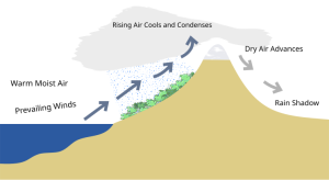
Another type of desert is found in the rain shadow created from prevailing winds blowing over mountain ranges. As the wind drives air up and over mountains, atmospheric moisture is released as snow or rain. Atmospheric pressure is lower at higher elevations, causing the moisture-laden air to cool. Cool air holds less moisture than hot air, and precipitation occurs as the wind rises up the mountain. After releasing its moisture on the windward side of the mountains, the dry air descends on the leeward, or downwind, side of the mountains to create an arid region with little precipitation called a rain shadow. Examples of rain-shadow deserts include the Western Interior Desert of North America and Atacama Desert of Chile, which is the Earth’s driest warm desert.
Finally, polar deserts, such as vast areas of the Antarctic and Arctic, are created from sinking cold air that is too cold to hold much moisture. Although they are covered with ice and snow, these deserts have very low average annual precipitation. As a result, Antarctica is Earth’s driest continent.

Video 13.1: Rain shadow
If you are using an offline version of this text, access this YouTube video via the QR code.
13.1.1 Atmospheric Circulation
Geographic location, atmospheric circulation, and the Earth’s rotation are the primary causal factors of deserts. Solar energy converted to heat is the engine that drives the circulation of air in the atmosphere and water in the oceans. The strength of the circulation is determined by how much energy is absorbed by the Earth’s surface, which in turn is dependent on the average position of the Sun relative to the Earth. In other words, the Earth is heated unevenly depending on latitude and angle of incidence. Latitude is a line circling the Earth parallel to the equator and is measured in degrees. The equator is 0°, and the North and South Poles are 90° N and 90° S, respectively (see Figure 13.4 for a diagram of generalized atmospheric circulation on Earth). Angle of incidence is the angle made by a ray of sunlight shining on the Earth’s surface. Tropical zones are located near the equator, where the latitude and angle of incidence are close to 0°, and receive high amounts of solar energy. The poles, which have latitudes and angles of incidence approaching 90°, receive little or almost no energy.
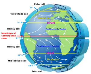
The figure shows the generalized air circulation within the atmosphere. Three cells of circulating air span the space between the equator and poles in both hemispheres, the Hadley cell, the Ferrel or midlatitude cell, and the polar cell. In the Hadley cell, located over the tropics and closest to the equatorial belt, the Sun heats the air and causes it to rise. The rising air cools and releases its contained moisture as tropical rain. The rising dried air spreads away from the equator and toward the North and South Poles, where it collides with dry air in the Ferrel cell. The combined dry air sinks back to the Earth at 30° latitude. This sinking drier air creates belts of predominantly high pressure at approximately 30° north and south of the equator, called the horse latitudes. Arid zones between 15° and 30° north and south of the equator thus exist, within which desert conditions predominate. The descending air flowing north and south in the Hadley and Ferrel cells also creates prevailing winds called trade winds near the equator and westerlies in the temperate zone. Note the arrows indicating general directions of winds in these zones.
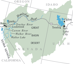
Other deserts, like the Great Basin Desert that covers parts of Utah and Nevada, owe at least part of their origin to other atmospheric phenomena. The Great Basin Desert, while somewhat affected by sinking air effects from global circulation, is a rain-shadow desert. As westerly moist air from the Pacific rises over the Sierra Nevadas and other mountains, it cools and loses moisture as condensation and precipitation on the upwind, rainy side of the mountains.
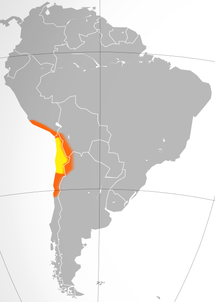
One of the driest places on Earth is the Atacama Desert of northern Chile. The Atacama Desert occupies a strip of land along Chile’s coast just north of latitude 30°S, at the southern edge of the trade-wind belt. The desert lies west of the Andes Mountains, in the rain shadow created by prevailing trade winds blowing west. As this warm moist air crossing the Amazon basin meets the eastern edge of the mountains, it rises, cools, and precipitates much of its water out as rain. Once over the mountains, the cool, dry air descends onto the Atacama Desert. Onshore winds from the Pacific are cooled by the Peru (Humboldt) ocean current. This super-cooled air holds almost no moisture and, with these three factors, some locations in the Atacama Desert have received no measured precipitation for several years. This desert is the driest nonpolar location on Earth.
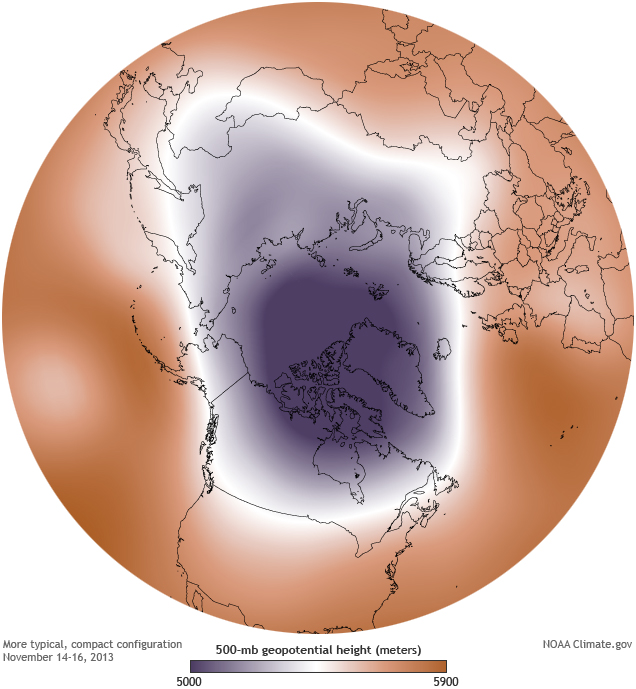
Notice in Figure 13.7 that the polar regions are also areas of predominantly high pressure created by descending cold dry air, the polar cells. As with the other cells, cold air, which holds much less moisture than warm air, descends to create polar deserts. This is why historically, land near the North and South Poles has always been so dry.
13.1.2 Coriolis Effect

The Earth rotates toward the east, where the sun rises. Think of spinning a weight on a string around your head. The speed of the weight depends on the length of the string. The speed of an object on the rotating Earth depends on its horizontal distance from the Earth’s axis of rotation. Higher latitudes are a smaller distance from the Earth’s rotational axis and therefore do not travel as fast eastward as lower latitudes that are closer to the equator. When a fluid like air or water moves from a lower latitude to a higher latitude, the fluid maintains its momentum from moving at a higher speed, so it will travel relatively faster eastward than the Earth beneath at the higher latitudes. This factor causes deflection of movements that occur in north-south directions.
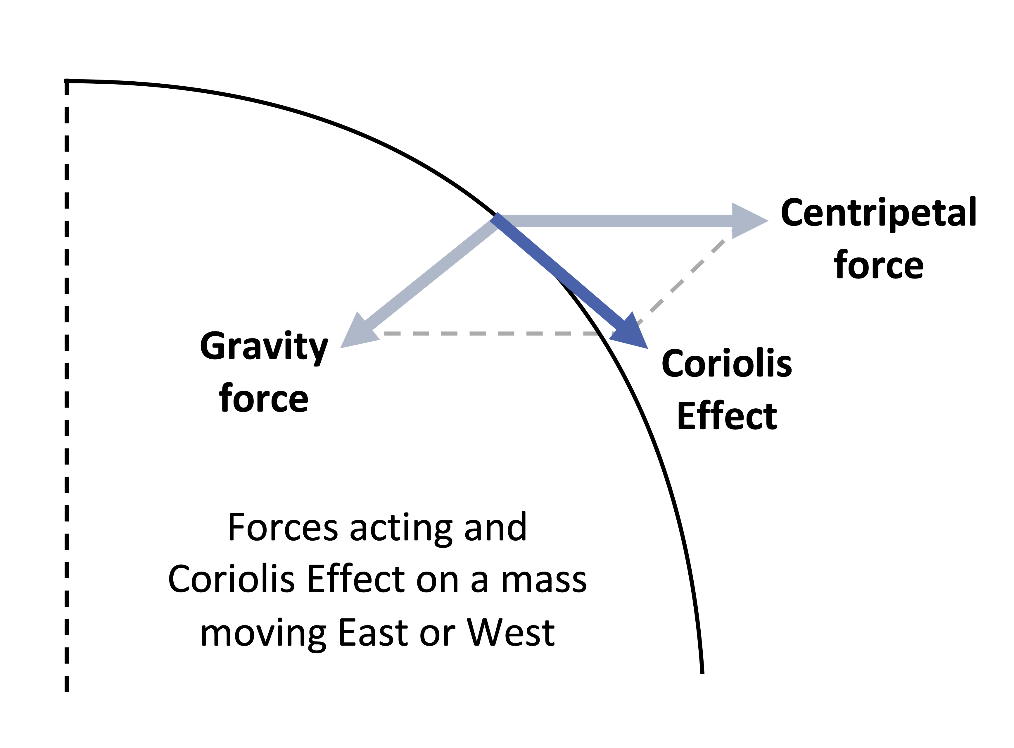
Another factor in the Coriolis effect also causes deflection of east-west movement due to the angle between the centripetal effect of Earth’s spin and gravity pulling toward the Earth’s center (see Figure 13.9). This produces a net deflection toward the equator. The total Coriolis deflection on a mass moving in any direction on the rotating Earth results from a combination of these two factors.
Since each hemisphere has three atmospheric cells moving respectively north and south relative to the Earth beneath them, the Coriolis effect deflects these moving air masses to the right in the Northern Hemisphere and to the left in the Southern Hemisphere. The Coriolis effect also deflects moving masses of water in the ocean currents.
For example, in the Northern Hemisphere Hadley cell, the lower altitude air currents are flowing south toward the equator. These are deflected to the right (or west) by the Coriolis effect. This deflected air generates the prevailing trade winds that European sailors used to cross the Atlantic Ocean and reach South America and the Caribbean Islands in their tall ships. This air movement is mirrored in the Hadley cell in the Southern Hemisphere; the lower-altitude air current flowing toward the equator is deflected to the left, creating trade winds that blow to the northwest.
In the northern Ferrel, or midlatitude, cell, surface air currents flow from the horse latitudes (latitude 30°) toward the North Pole, and the Coriolis effect deflects them toward the east or to the right, producing the zone of westerly winds. In the Southern Hemisphere Ferrel cell, the poleward flowing surface air is deflected to the left and flows southeast, creating the Southern Hemisphere westerlies.
Another Coriolis-generated deflection produces the polar cells. At 60° north and south latitude, relatively warmer rising air flows poleward, cooling and converging at the poles where it sinks in the polar high. This sinking dry air creates the polar deserts, the driest deserts on Earth. The persistence of ice and snow is a result of cold temperatures at these dry locations.
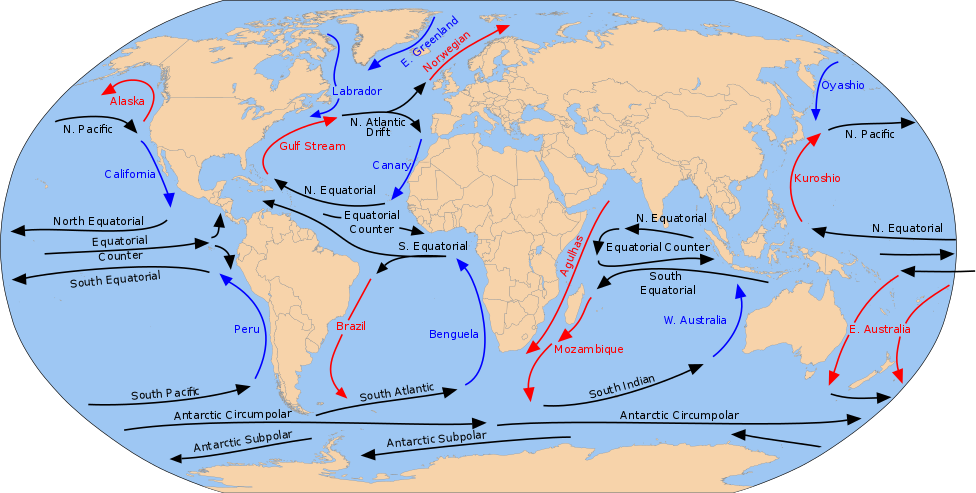
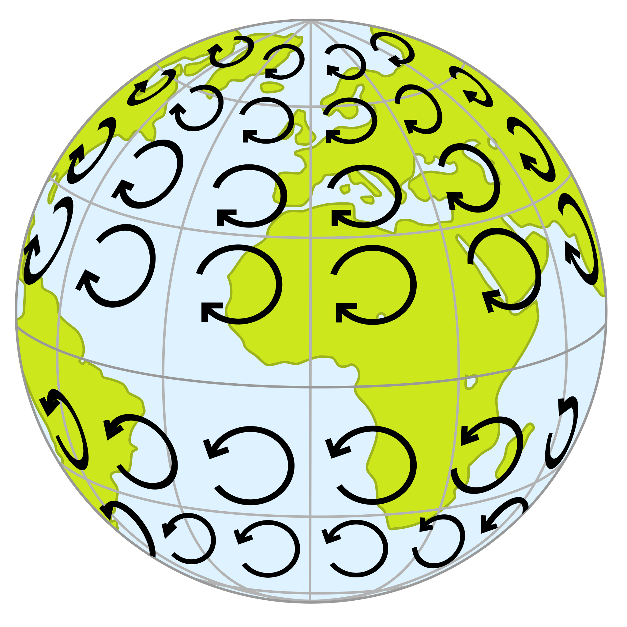
The Coriolis effect operates on all motions on the Earth. Artillerymen must take the Coriolis effect into account on ballistic trajectories when making long-distance targeting calculations. Geologists note how its effect on air and oceanic currents creates deserts in designated zones around the Earth as well as creating the surface currents in the ocean. The Coriolis effect causes the ocean gyres to turn clockwise in the Northern Hemisphere and counterclockwise in the Southern. It also affects weather by creating high-altitude, polar jet streams that sometimes push lobes of cold arctic air into the temperate zone, down to as far as latitude 30° from the usual 60°. It also causes low-pressure systems and intense tropical storms to rotate counterclockwise in the Northern Hemisphere and clockwise in the Southern Hemisphere.

Video 13.2: The Coriolis effect
If you are using an offline version of this text, access this YouTube video via the QR code.

Take this quiz to check your comprehension of this section.
If you are using an offline version of this text, access the quiz for Section 13.1 via the QR code.
13.2 Desert Processes
13.2.1 Desert Weathering and Erosion
Weathering takes place in desert climates by the same means as other climates, only at a slower rate. While higher temperatures typically spur faster chemical weathering, water is the main agent of weathering, and lack of water slows both mechanical and chemical weathering. Low precipitation levels also mean less runoff as well as ice wedging. When precipitation does occur in the desert, it is often heavy and may result in flash floods in which a lot of material may be dislodged and moved quickly.
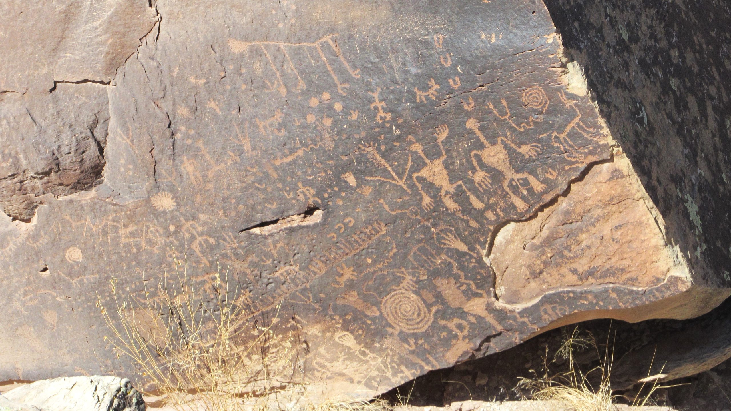
One unique weathering product in deserts is desert varnish. Also known as desert patina or rock rust, this is thin dark-brown layers of clay minerals and iron and manganese oxides that form on very stable surfaces within arid environments. The exact way this material forms is still unknown, though cosmogenic and biologic mechanisms have been proposed.
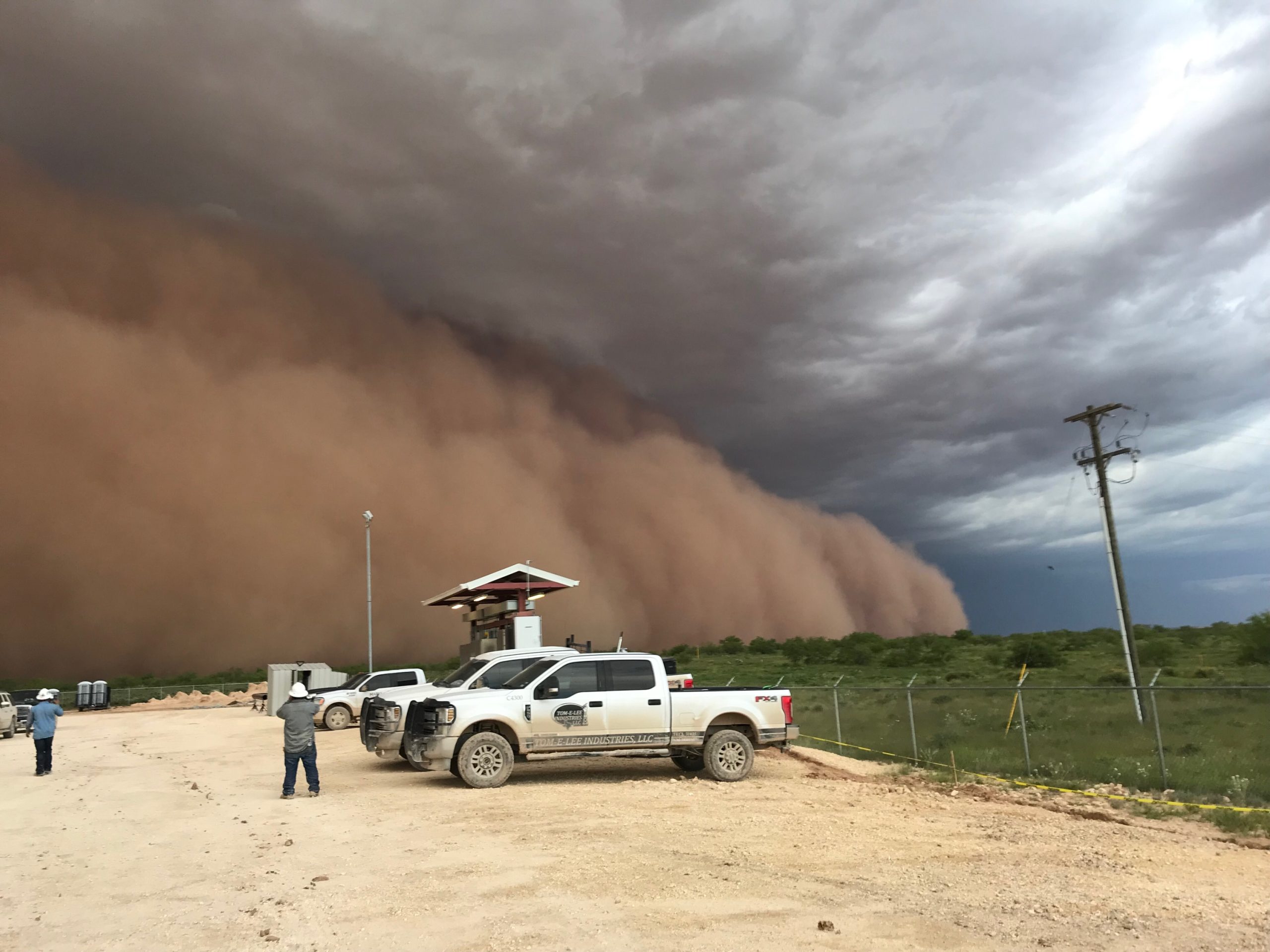
While water is still the dominant agent of erosion in most desert environments, wind is a notable agent of weathering and erosion in many deserts. This includes suspended sediment traveling in haboobs, or large dust storms, that frequent deserts. Deposits of windblown dust are called loesses. Loess deposits cover wide areas of the Midwestern United States, much of it from rock flour that melted out of the ice sheets during the last ice age. Loess was also blown from desert regions in the West. Possessing lower energy than water, wind transport nevertheless moves sand, silt, and dust. As noted in Chapter 11, the load carried by a fluid (air is a fluidlike water) is distributed among bedload and suspended load. As with water, in wind these components depend on wind velocity.
Sand-sized material moves by a process called saltation in which sand grains are lifted into the moving air and carried a short distance, where they drop and splash into the surface, dislodging other sand grains that are then carried a short distance and splash, dislodging still others.
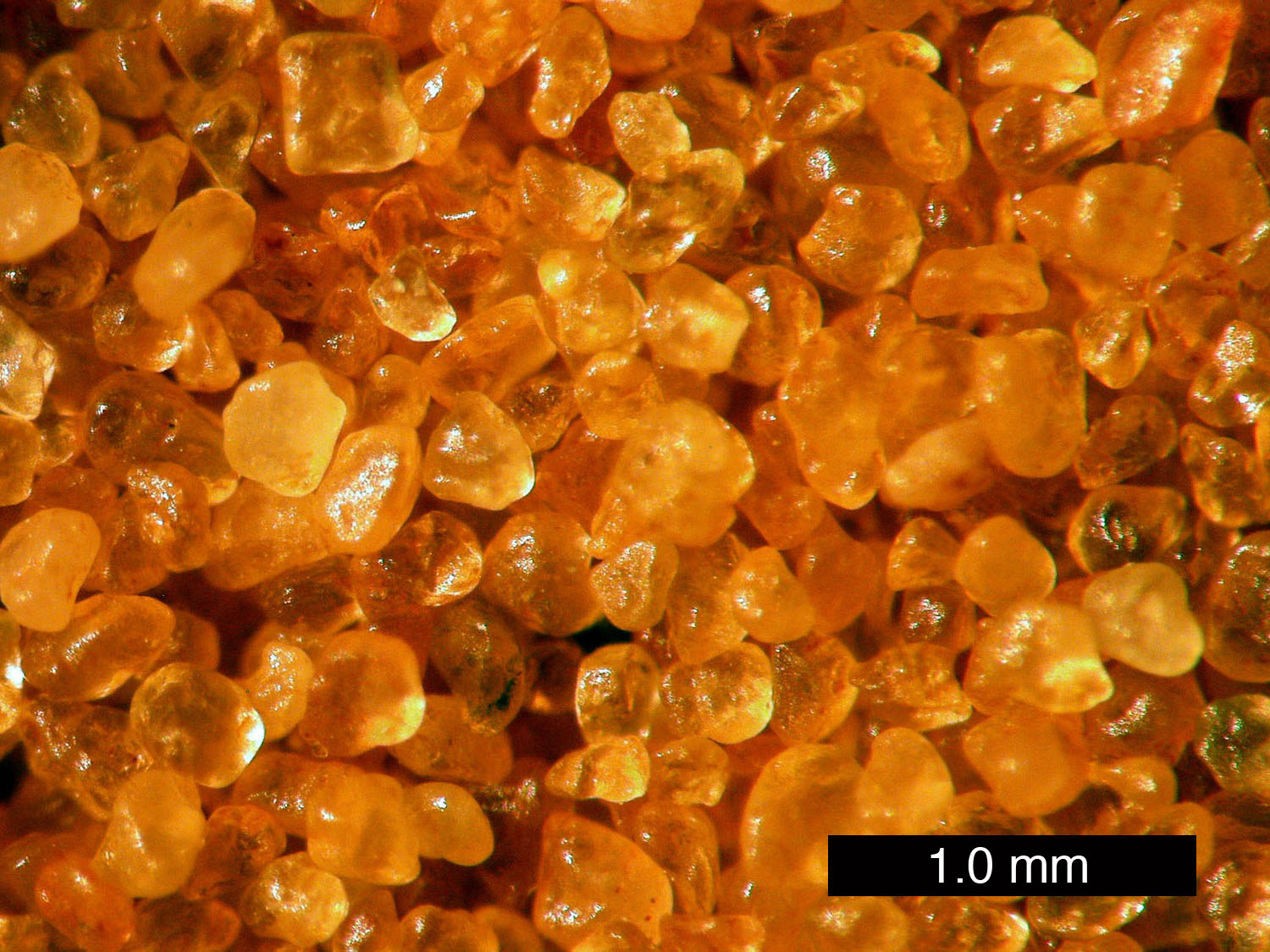
Since saltating sand grains are constantly impacting other sand grains, windblown sand grains are commonly quite well rounded, with frosted surfaces. Saltation is a cascading effect of sand movement, creating a zone of windblown sand up to a meter or so above the ground. This zone of saltating sand is a powerful erosive agent in which bedrock features are effectively sandblasted. The fine-grained suspended load is effectively sorted from the sand near the surface, carrying the silt and dust into haboobs. Wind is thus an effective sorting agent separating sand and dust-sized (≤70 µm) particles (see Chapter 5). When wind velocity is high enough to slide or roll materials along the surface, the process is called creep.
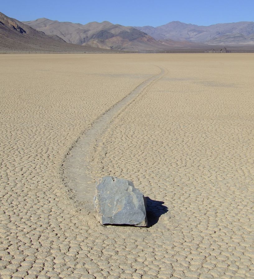
One extreme version of sediment movement was shrouded in mystery for years: sliding stones. Also called sailing stones and sliding rocks, these are large boulders that move along flat surfaces in deserts, leaving trails. This includes the famous example of the Racetrack Playa in Death Valley National Park, California. For years, scientists and enthusiasts attempted to explain their movement, with few definitive results. In recent years, several experimental and observational studies have confirmed that the stones, embedded in thin layers of ice, are propelled by friction from high winds. These studies include measurements of actual movement, as well as recreations of the conditions, with resulting movement in the lab.
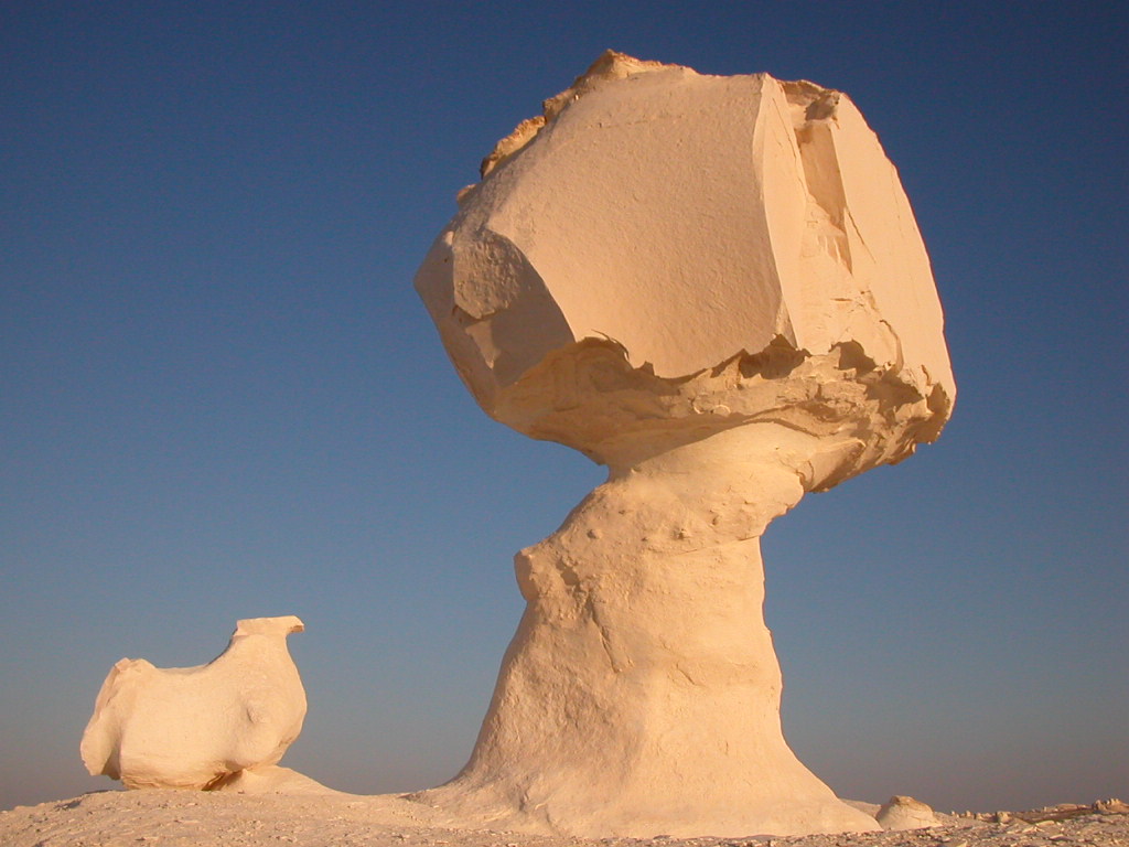
The zone of saltating sand is an effective agent of erosion through sand abrasion. A bedrock outcrop which has such a sandblasted shape is called a yardang. Rocks and boulders lying on the surface may be blasted and polished by saltating sand. When predominant wind directions shift, multiple sandblasted and polished faces may appear. Such wind-abraded desert rocks are called ventifacts.
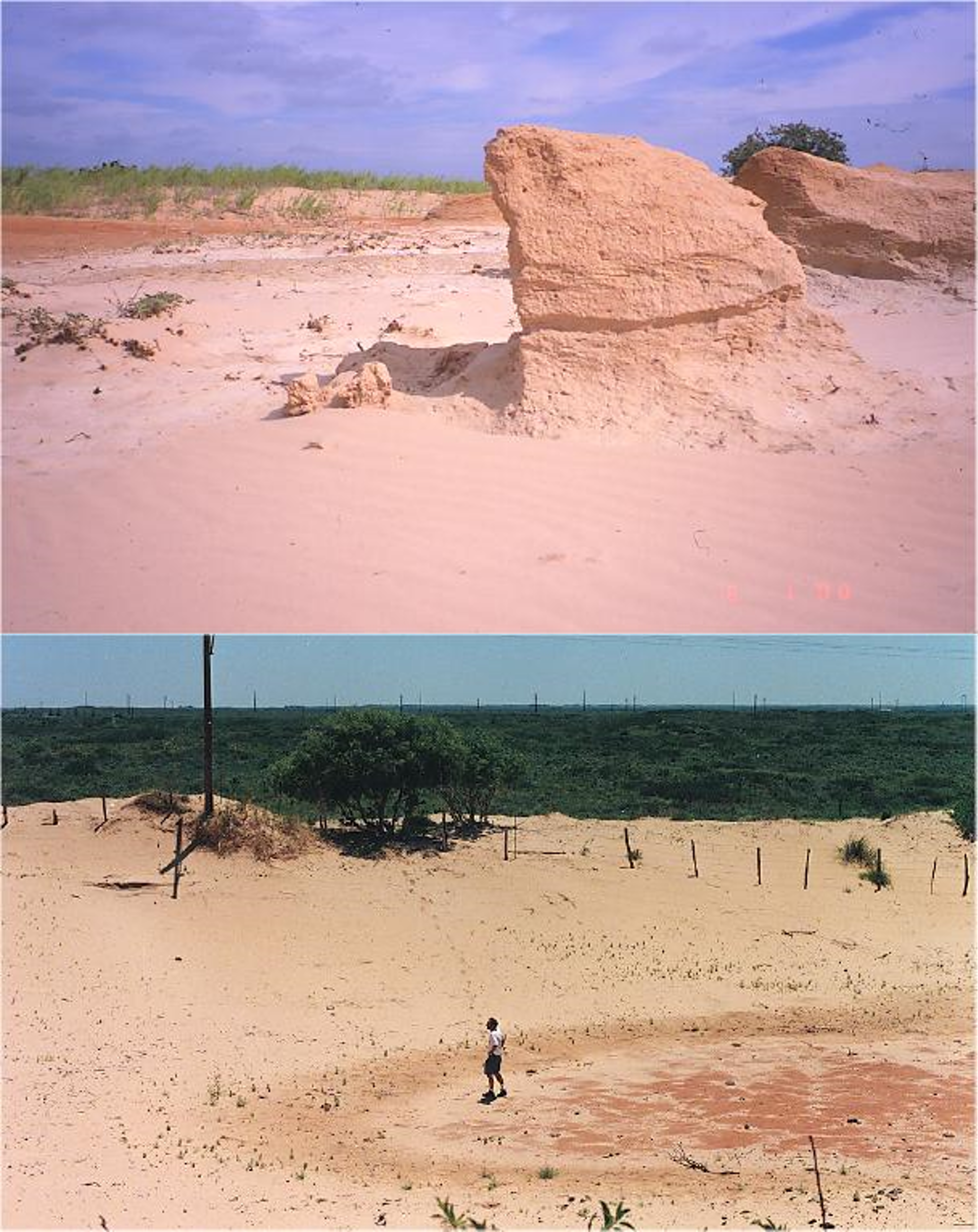
In places with sand and silt accumulations, clumps of vegetation often anchor sediment on the desert surface. Yet, winds may be sufficient to remove materials not anchored by vegetation. The bowl-shaped depression remaining on the surface is called a blowout.
13.2.2 Desert Landforms
In the American Southwest, as streams emerge into the valleys from the adjacent mountains, they create desert landforms called alluvial fans. When a stream emerges from the narrow canyon, the flow is no longer constrained by the canyon walls and spreads out. At the lower slope angle, the water slows down and drops its coarser load. As the channel fills with this conglomeratic material, the stream is deflected around it. This deposited material deflects the stream into a system of radial distributary channels in a process similar to a delta’s formation by a river entering a body of water. This process develops a system of radial distributaries and constructs a fan-shaped alluvial fan.
Alluvial fans continue to grow and may eventually coalesce with neighboring fans to form an apron of alluvium along the mountain front called a bajada.
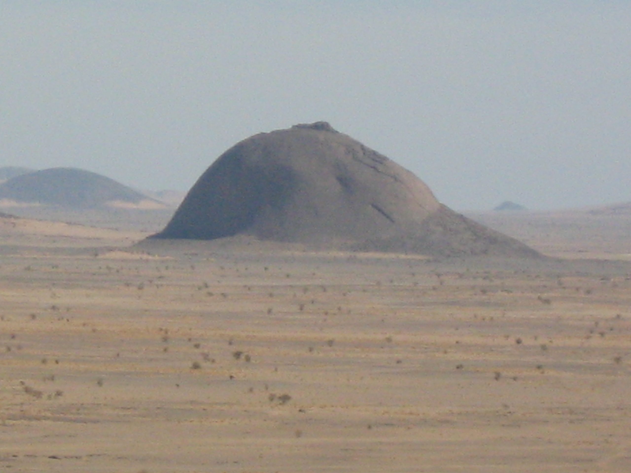
As the mountains erode away and their sediment accumulates first in alluvial fans, then bajadas, the mountains eventually are buried in their own erosional debris. Such buried mountain remnants are called inselbergs, “island mountains,” as first described by the German geologist Wilhelm Bornhardt (1864–1946).
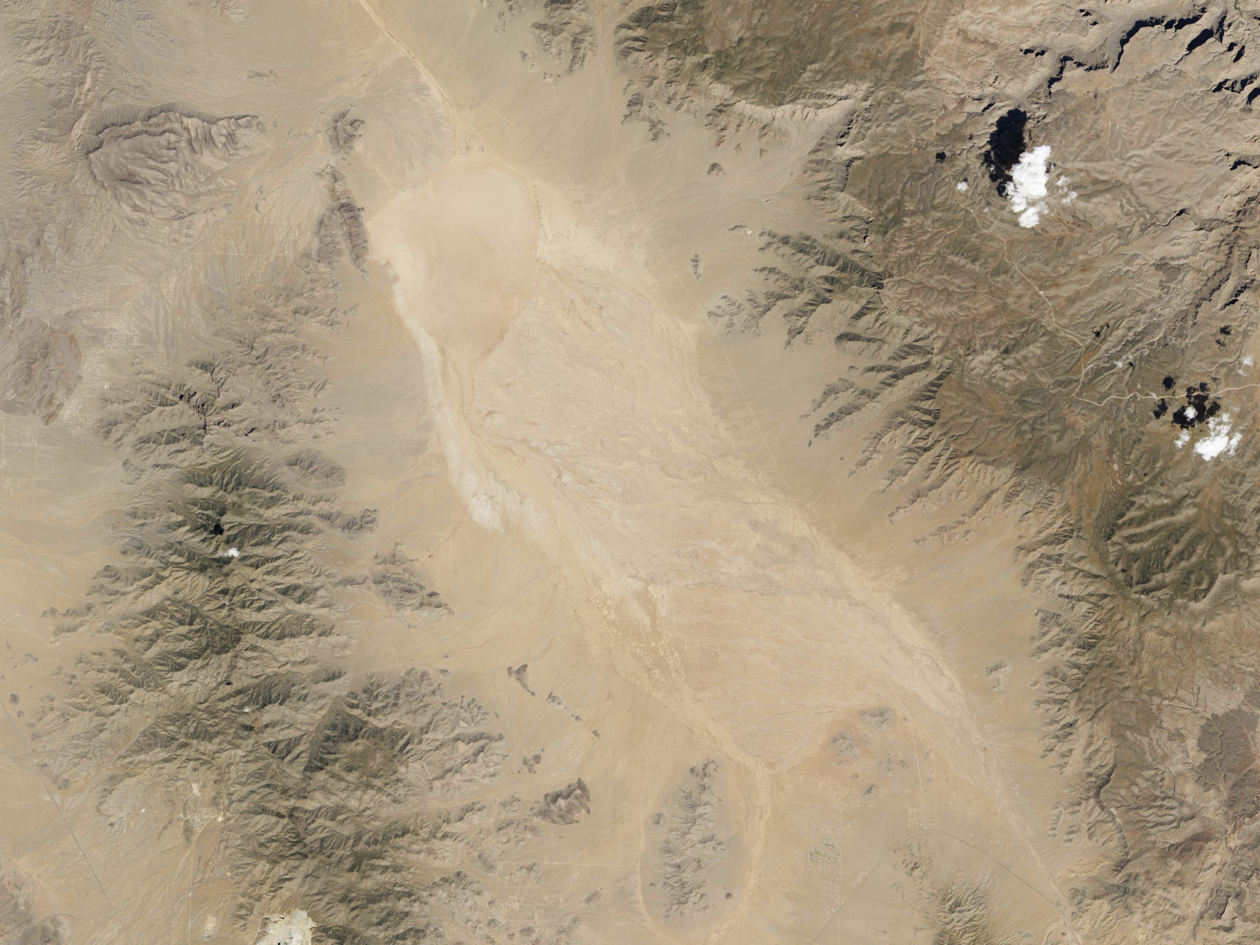
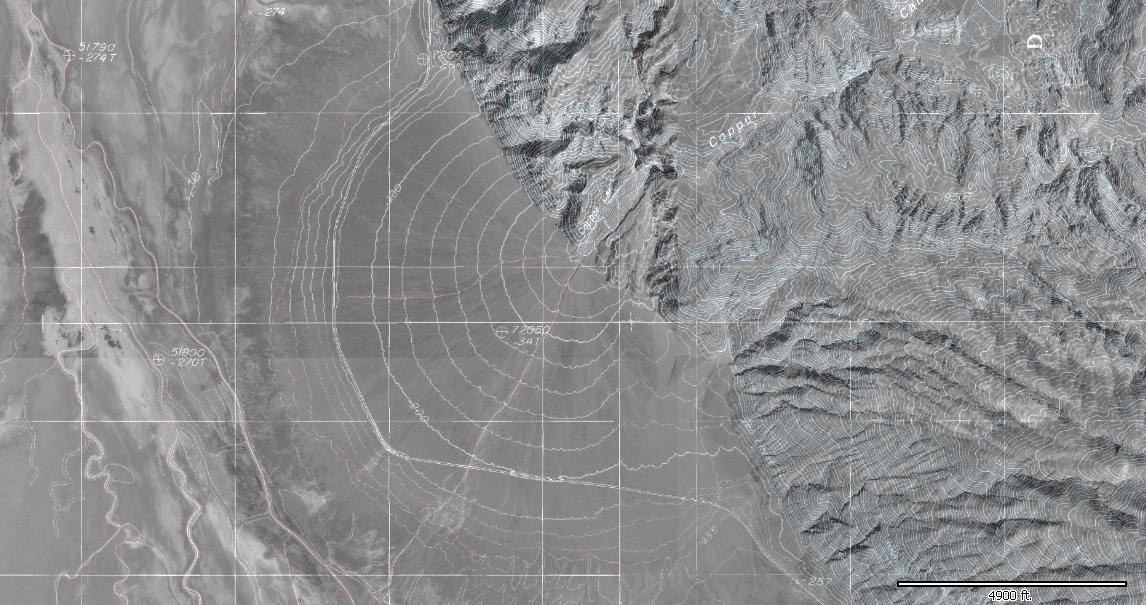
Where the desert valley is an enclosed basin—i.e., streams entering it do not drain out—the water is removed by evaporation and a dry lake bed called a playa is formed.
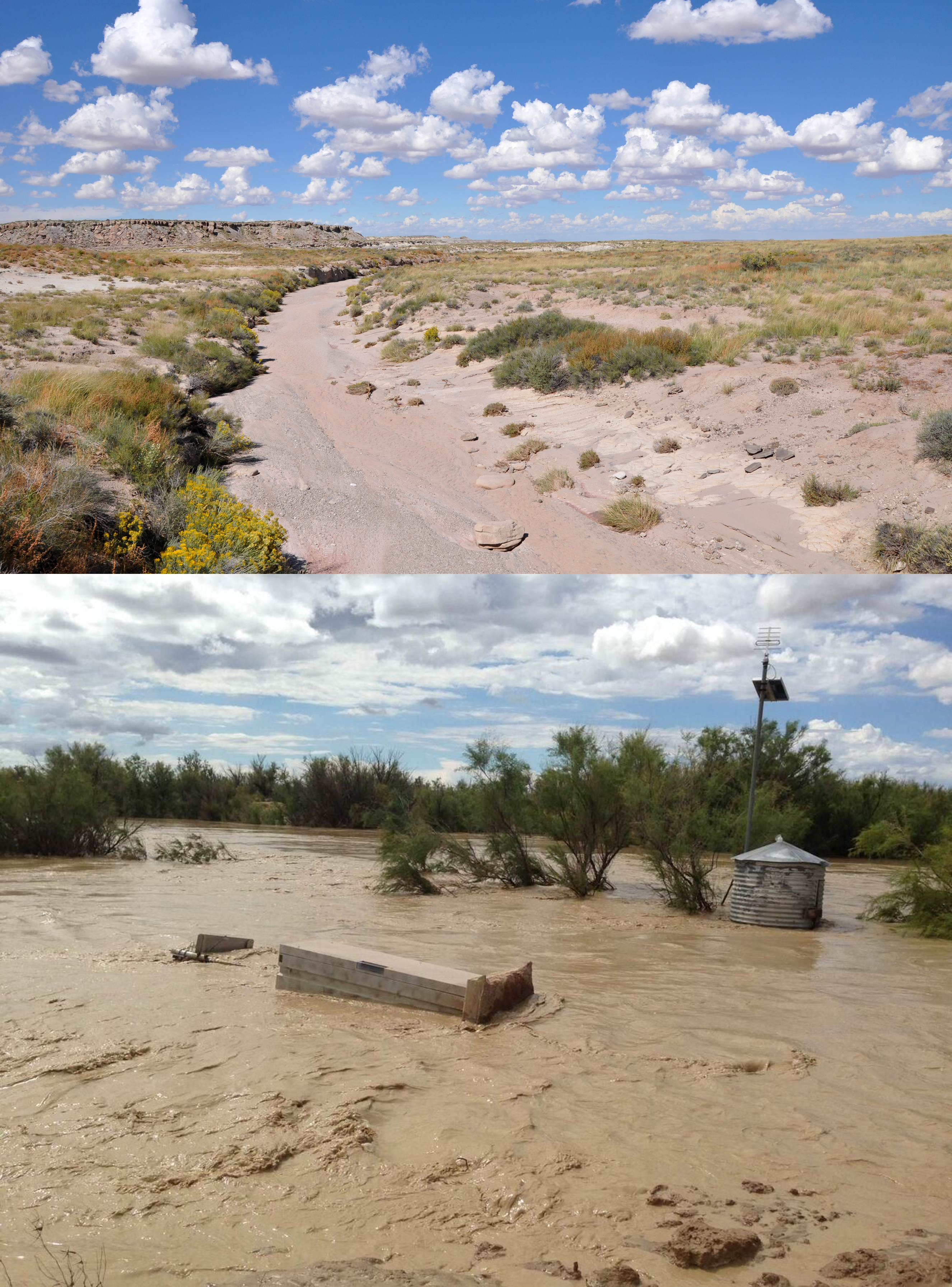
Playas are among the flattest of all landforms. Such a dry lake bed may cover a large area and be filled after a heavy thunderstorm to only a few inches deep. Playa lakes and desert streams that contain water only after rainstorms are called intermittent or ephemeral. Because of intense thunderstorms, the volume of water transported by ephemeral drainage in arid environments can be substantial during a short period of time. Desert soil structures lack organic matter that promotes infiltration by absorbing water. Instead of percolating into the soil, the runoff compacts the ground surface, making the soil hydrophobic (i.e., water-repellant). Because of this hardpan surface, ephemeral streams may gather water across large areas, suddenly filling with water from storms many miles away.
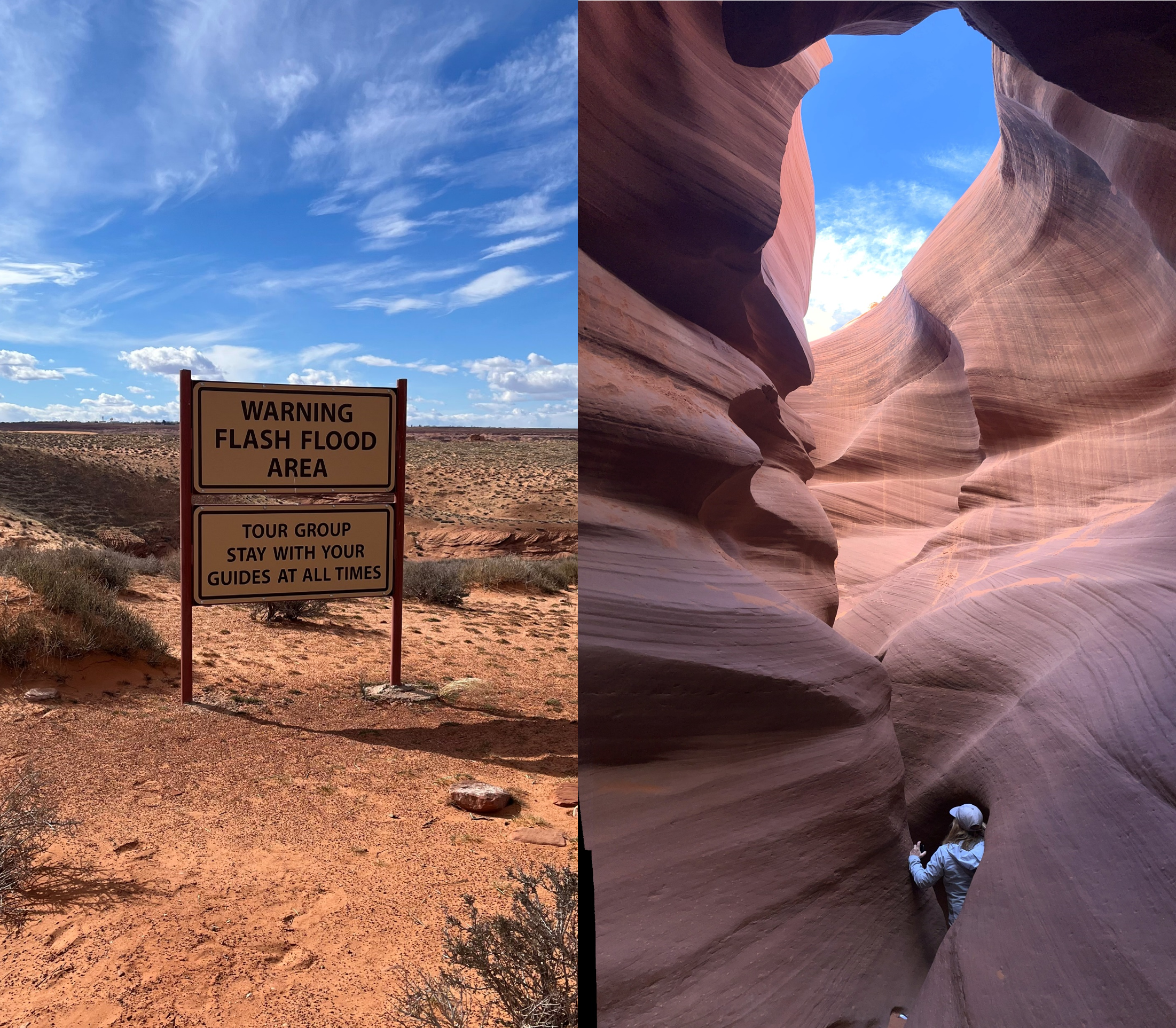
High-volume ephemeral flows, called flash floods, may move as sheet flows or sheetwash; they can also be channeled through normally dry arroyos or canyons. Flash floods are a major factor in desert deposition. Dry channels can fill quickly with ephemeral drainage, creating a mass of water and debris that charges down the arroyo, even overflowing the banks. Flash floods pose a serious hazard for desert travelers because the storm activity feeding the runoff may be miles away. People hiking or camping in arroyos that have been bone dry for months or years have been swept away by sudden flash floods.
13.2.3 Sand
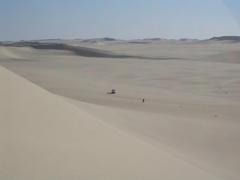
The popular concept of a typical desert is a broad expanse of sand. Geologically, deserts that are defined by a lack of water and arid regions resembling seas of sand belong to the category of desert called an erg. An erg consists of fine-grained, loose sand grains, often blown by wind, or aeolian forces, into dunes. Probably the best known erg is the Rub’ al Khali, which means empty quarter, of the Arabian Peninsula. Ergs are also found in the Great Sand Dunes National Park (Colorado), Little Sahara Recreation Area (Utah), White Sands National Monument (New Mexico), and parts of Death Valley National Park (California). Ergs are not restricted to deserts but may form anywhere there is a substantial supply of sand, including as far north as 60° N in Saskatchewan, Canada, in the Athabasca Sand Dunes Provincial Park. Coastal ergs exist along lakes and oceans as well, and examples are found in Oregon, Michigan, and Indiana.
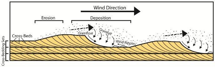
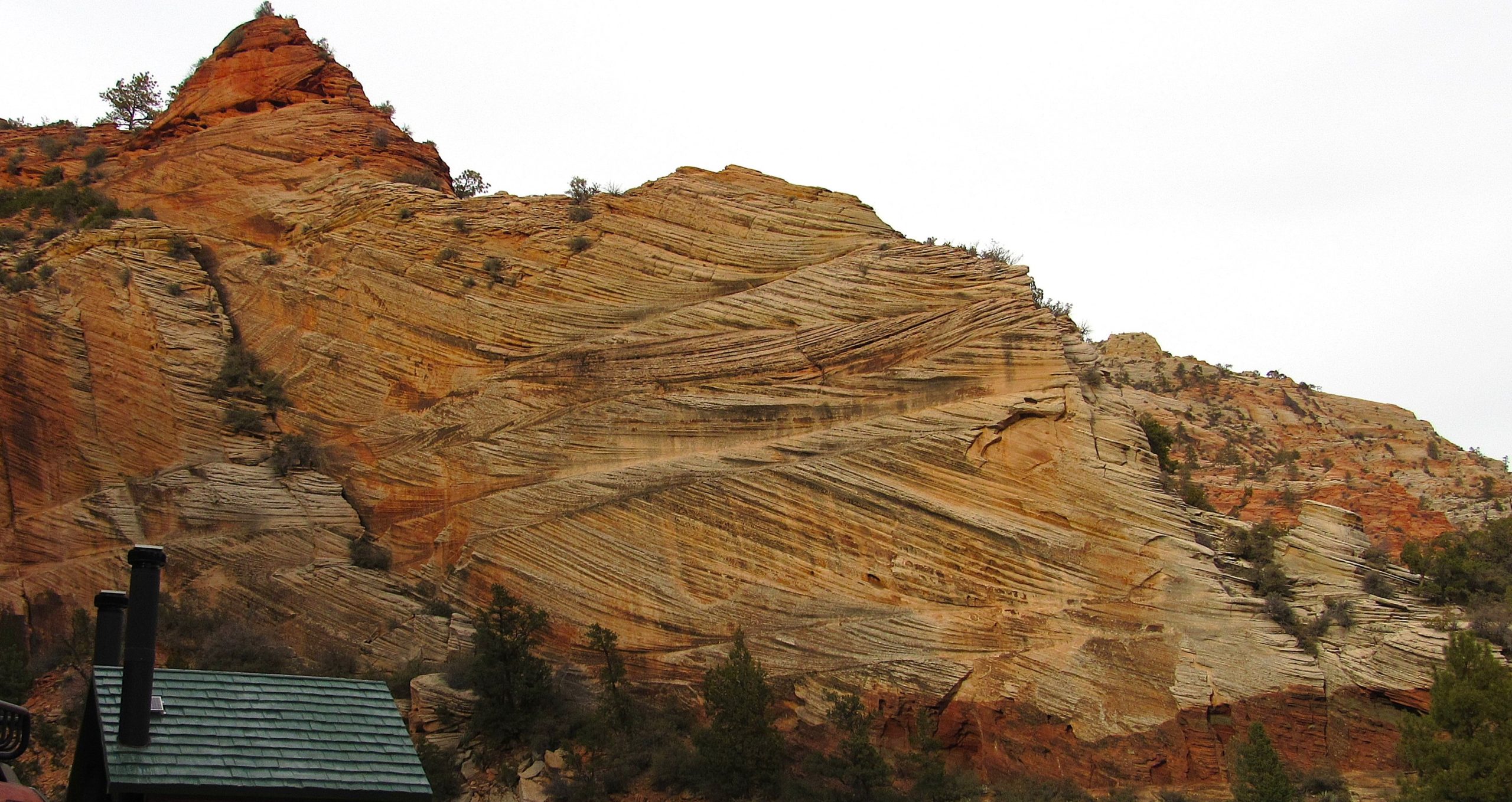
An internal cross section of a sand dune shows a feature called cross-bedding. As wind blows up the windward side of the dune, it carries sand to the dune crest, depositing layers of sand parallel to the windward (or “stoss”) side. The sand builds up the crest of the dune and pours over the top until the leeward (downwind or slip) face of the dune reaches the angle of repose, the maximum angle which will support the slip face. Dunes are unstable features and move as the sand erodes from the stoss side and continues to drop down the leeward side, covering previous stoss and slip-face layers and creating the cross-beds. Mostly, these are reworked over and over again, but occasionally, the features are preserved in a depression, then lithified. Shifting wind directions and abundant sand sources create chaotic patterns of cross-beds like those seen in Zion National Park of Utah.
In the Mesozoic Era, Utah was covered by a series of ergs, with the thickest being in southern Utah, which lithified into sandstone (see Chapter 5). Perhaps the best known of these sandstone formations is the Navajo Sandstone of Jurassic age. This sandstone formation consists of dramatic cliffs and spires in Zion National Park and covers a large part of the Colorado Plateau. In Arches National Park, a later series of sand dunes covered the Navajo Sandstone and lithified to become the Entrada Formation also during the Jurassic. Erosion of overlying layers exposed fins of the underlying Entrada Sandstone and carved out weaker parts of the fins forming the arches.
As the cements that hold the grains together in these modern sand cliffs disintegrate and the freed grains gather at the base of the cliffs and move down the washes, sand grains may be recycled and redeposited. These Mesozoic sand ergs may represent ancient quartz sands recycled many times from igneous origins in the early Precambrian, just passing now through another cycle of erosion and deposition. An example of this is Coral Pink Sand Dunes State Park in southwestern Utah, which contains sand that is being eroded from the Navajo Sandstone to form new dunes.
13.2.4 Dune Types
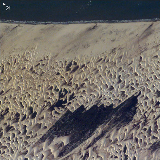
Dunes are complex features formed by a combination of wind direction and sand supply, in some cases interacting with vegetation. There are several types of dunes representing variables of wind direction, sand supply, and vegetative anchoring. Crescent-shaped barchan dunes form where sand supply is limited and there is a fairly constant wind direction. Barchans move downwind and develop a crescent shape with wings on either side of a dune crest. Barchans are known to actually move over homes, even towns.

Longitudinal dunes, or linear dunes, form where sand supply is greater and the wind blows a dominant direction in a back-and-forth manner. They may form ridges tens of meters high lined up with the predominant wind directions.
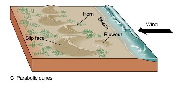
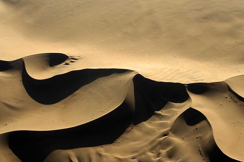
Parabolic dunes form where vegetation anchors parts of the sand and unanchored parts blow out. Parabolic dune shape may be similar to barchan dunes but usually reversed, and it is determined more by the anchoring vegetation than a strict parabolic form.
Star dunes form where the wind direction is variable in all directions. Sand supply can range from limited to quite abundant. It is the variation in wind direction that forms the star.

Take this quiz to check your comprehension of this section.
If you are using an offline version of this text, access the quiz for Section 13.2 via the QR code.
13.3 The Great Basin and the Basin and Range
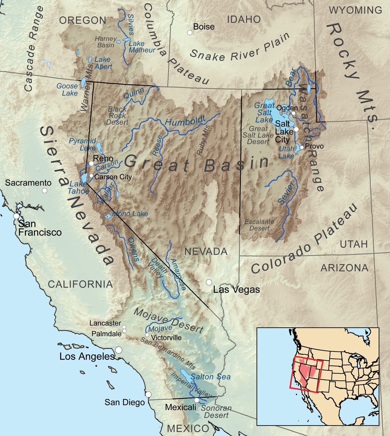
The Great Basin is the largest area of interior drainage in North America, meaning there is no outlet to the ocean and all precipitation remains in the basin or is evaporated. It covers western Utah, most of Nevada, and extends into southeastern California, southern Oregon, and southern Idaho. Because there is no outlet to the ocean, streams in the Great Basin deliver runoff to lakes and playas within the basin. A subregion within the Great Basin is the Basin and Range, which extends from the Wasatch Front in Utah west across Nevada to the Sierra Nevada Mountains of California. The basins and ranges referred to in the name are horsts and grabens, formed by normal fault blocks from crustal extension, as discussed in Chapters 2 and 9. The lithosphere of the entire area has stretched by a factor of about 2, meaning from end to end, the distance has doubled over the past 30 million years or so. Valleys without outlets form individual basins, each of which is filled with alluvial sediments leading into playa depositional environments. During the recent ice age, the climate was more humid, and while glaciers were forming in some of the mountains, pluvial lakes formed over large areas. During the ice age, valleys in much of western Utah and eastern Nevada were covered by Lake Bonneville. As the climate became arid after the ice age, Lake Bonneville dried, leaving as a remnant the Great Salt Lake in Utah.
The desert of the Basin and Range extends from about 35° to near 40° and results from a rain shadow effect created by westerly winds from the Pacific rising and cooling over the Sierras, becoming depleted of moisture by precipitation on the western side. The result is relatively dry air descending across Nevada and western Utah.
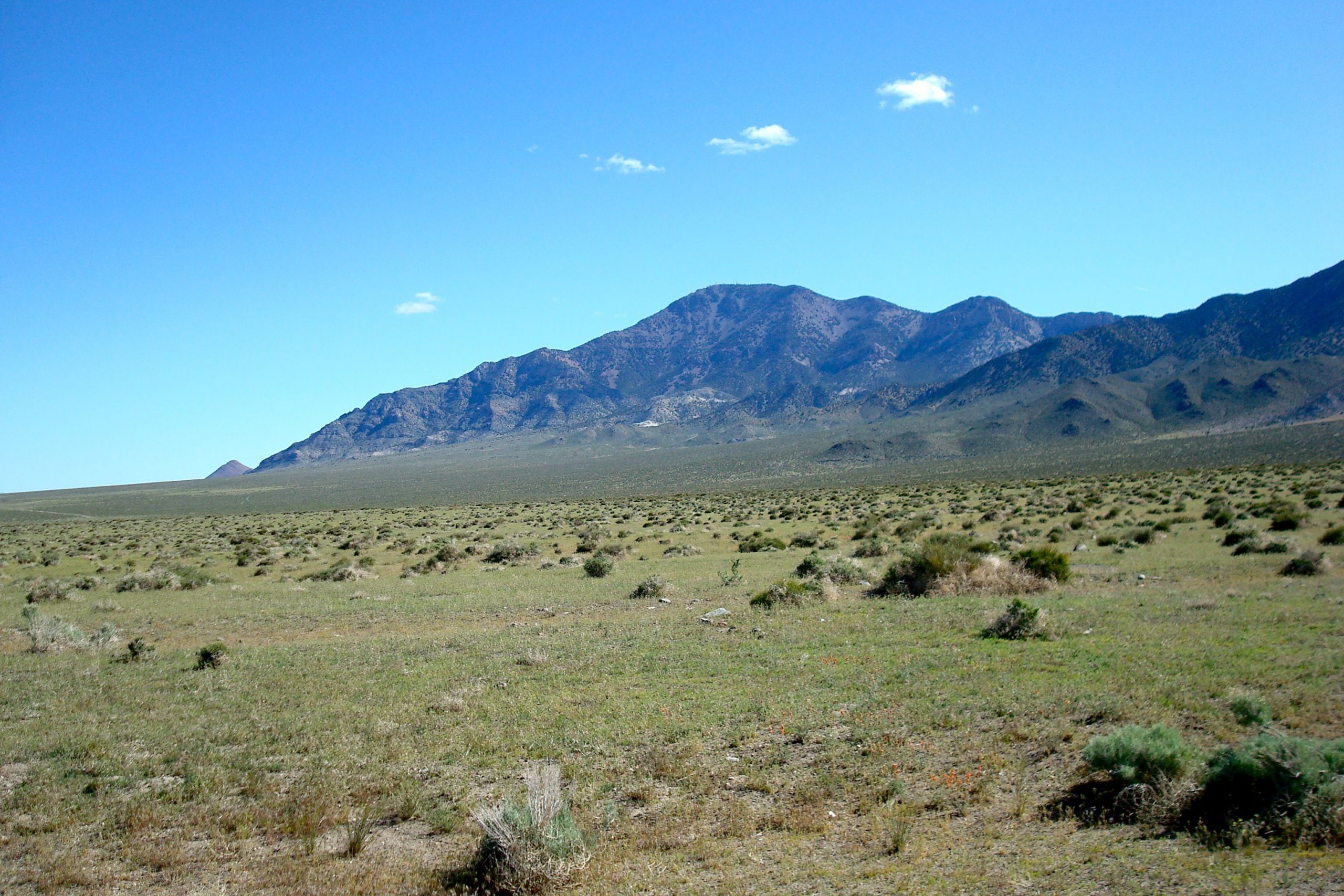
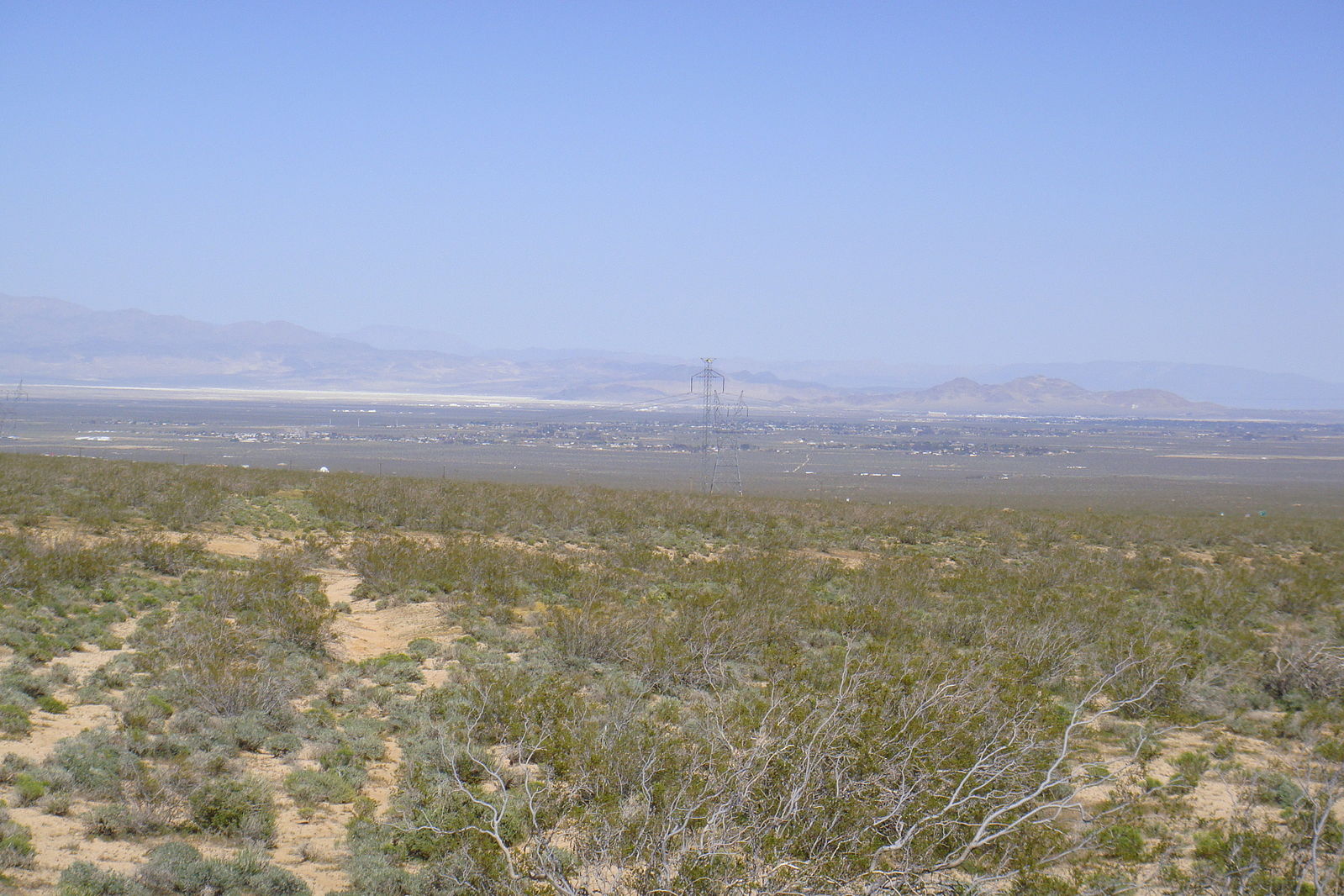
A journey from the Wasatch Front southwest to the Pacific Ocean will show stages of desert landscape evolution from the fault block mountains of Utah with sharp peaks and alluvial fans at the mouths of canyons, through landscapes in Southern Nevada with bajadas along the mountain fronts, to the landscapes in the Mojave Desert of California with subdued inselbergs sticking up through a sea of coalesced bajadas. These landscapes illustrate the evolutionary stages of desert landscape development.
13.3.1 Desertification
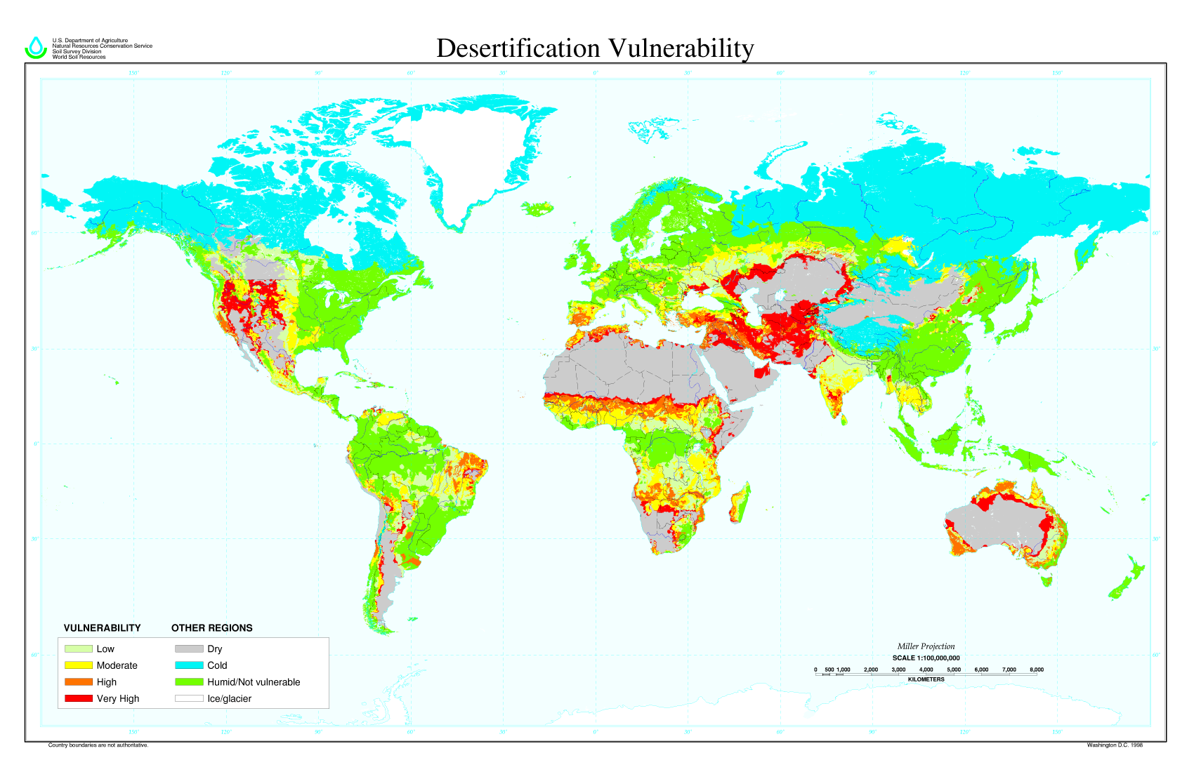
When previously arable land suitable for agriculture transforms into desert, this process is called desertification. Plants and humus-rich soil (see Chapter 5) promote groundwater infiltration and water retention. When an area becomes more arid due to changing environmental conditions, the plants and soil become less effective in retaining water, creating a positive feedback loop of desertification. This self-reinforcing loop spirals into increasingly arid conditions and further enlarges the desert regions.
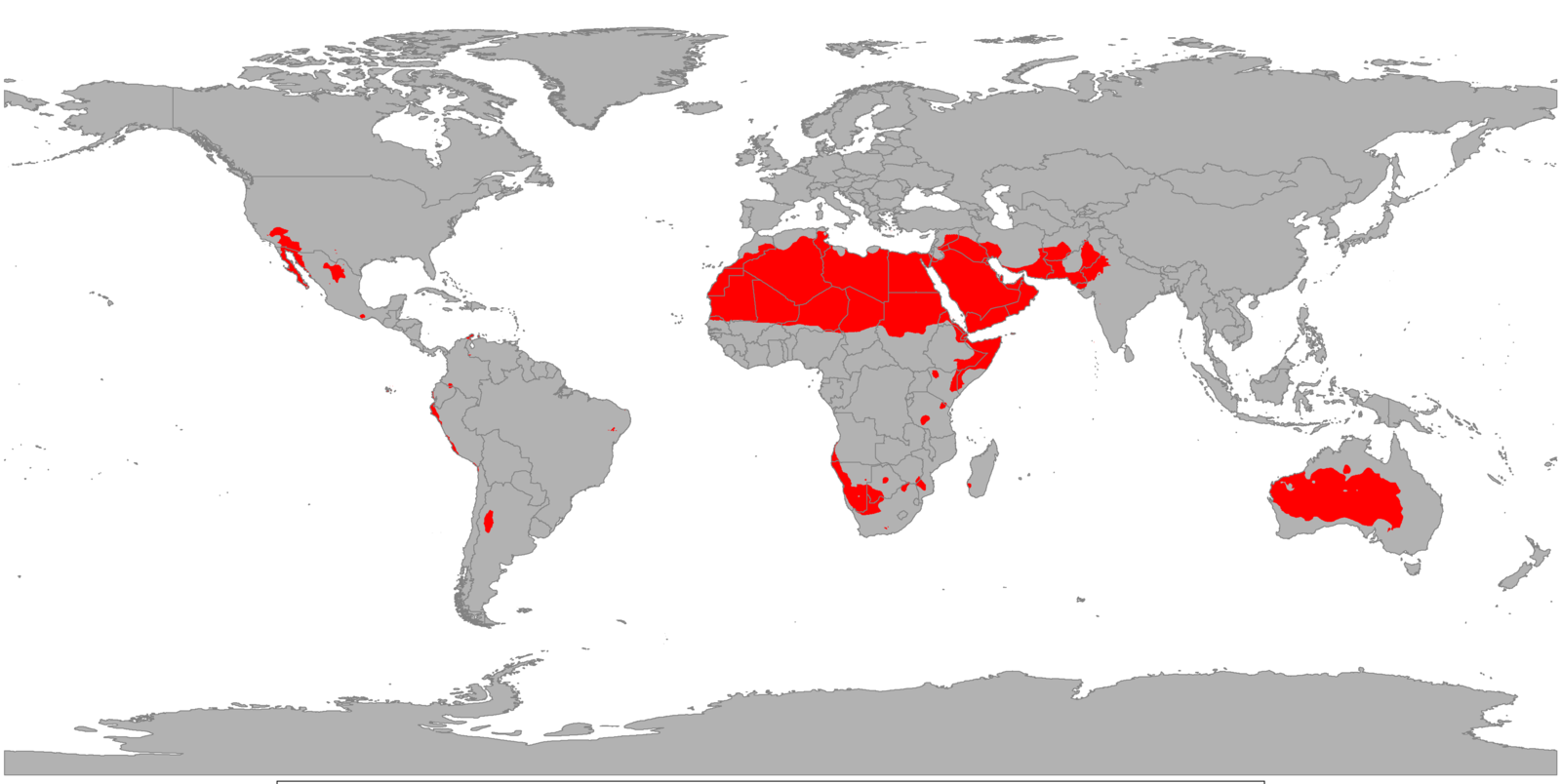
Desertification may be caused by human activities, such as unsustainable crop-cultivation practices, overgrazing by livestock, overuse of groundwater, and global climate change. Human-caused desertification is a serious worldwide problem. The world map figure above shows what areas are most vulnerable to desertification. Note the red and orange areas in the Western and Midwestern regions of the United States, which also cover large areas of arable land used for raising food crops and animals. The creation of the Dust Bowl in the 1930s (see Chapter 5) is a classic example of a high-vulnerability region impacted by human-caused desertification. As demonstrated in the Dust Bowl, conflicts may arise between agricultural practices and conservation measures. Mitigating desertification while allowing farmers to make a survivable living requires public and individual education to create community support and understanding of sustainable agriculture alternatives.

Take this quiz to check your comprehension of this section.
If you are using an offline version of this text, access the quiz for Section 13.3 via the QR code.
13.4 Glaciers
The Earth’s cryosphere, or ice, has a unique set of erosional and depositional features compared to its hydrosphere, or liquid water. This ice exists primarily in two forms, glaciers and icebergs. Glaciers are large accumulations of ice that exist year-round on the land surface. In contrast, masses of ice floating on the ocean are icebergs, although they may have had their origin in glaciers.
Glaciers cover about 10% of the Earth’s surface and are powerful erosional agents that sculpt the planet’s surface. These enormous masses of ice usually form in mountainous areas that experience cold temperatures and high precipitation. Glaciers also occur in low-lying areas such as Greenland and Antarctica that remain extremely cold year-round.
13.4.1 Glacier Formation
Glaciers form when repeated annual snowfall accumulates as deep layers of snow that are not completely melted in the summer. Thus there is an accumulation of snow that builds up into deep layers. Perennial snow is a snow accumulation that lasts all year. A thin accumulation of perennial snow is a snow field. Over repeated seasons of perennial snow, the snow settles, compacts, and bonds with underlying layers. The amount of void space between the snow grains diminishes. As the old snow gets buried by more new snow, the older snow layers compact into firn, or névé, a granular mass of ice crystals. As the firn continues to be buried, compressed, and recrystallizes, the void spaces become smaller and the ice becomes less porous, eventually turning into glacier ice. Solid glacial ice still retains a fair amount of void space that traps air. These small air pockets provide records of the past atmosphere composition.
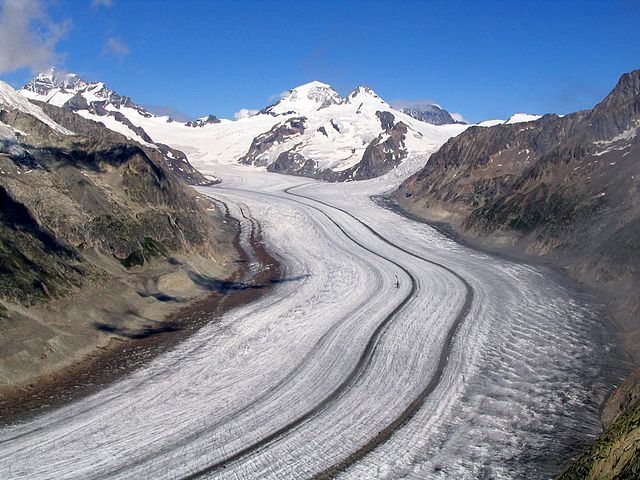
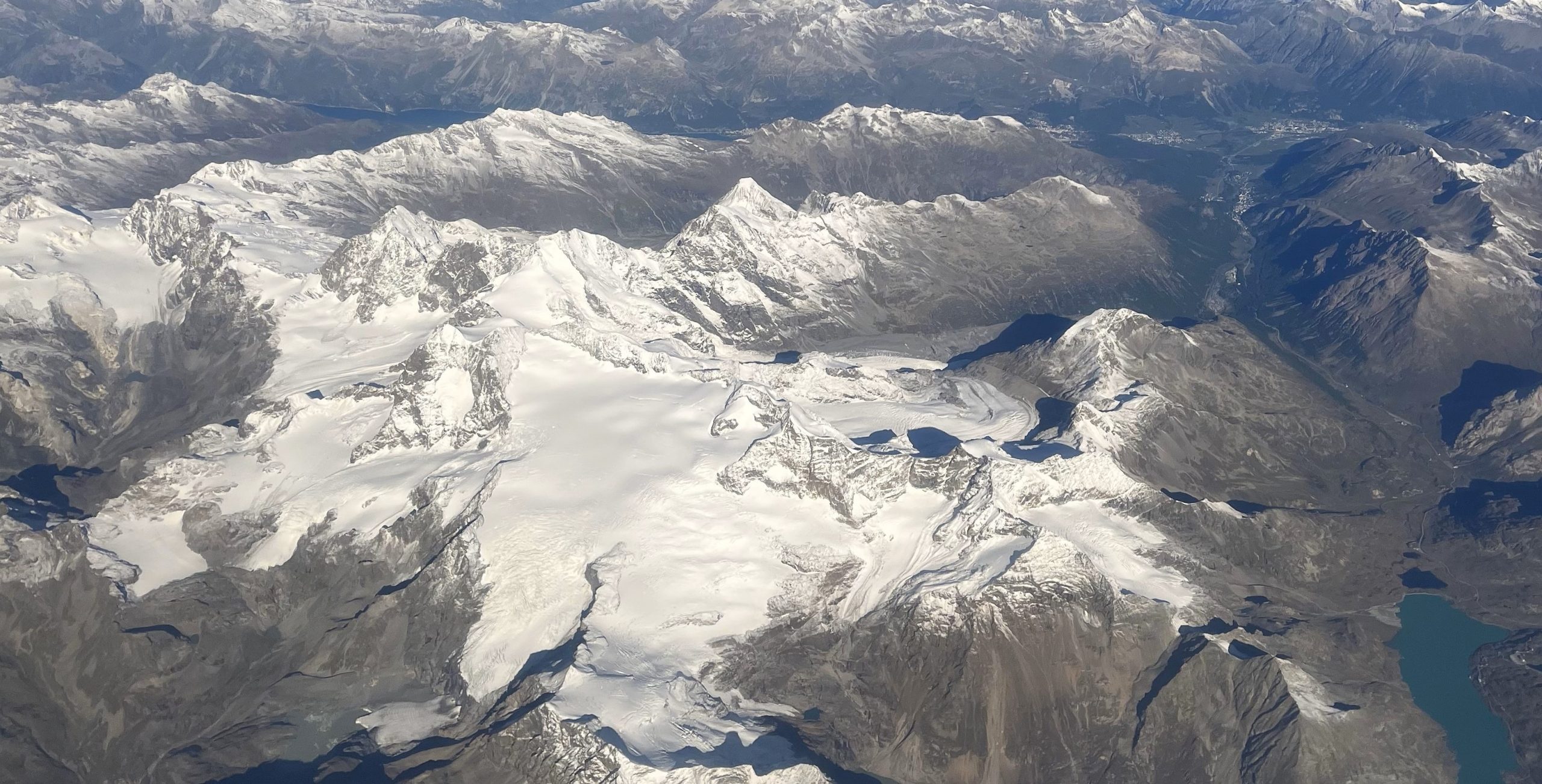
There are three general types of glaciers: alpine or valley glaciers, ice sheets, and ice caps. Most alpine glaciers are located in the world’s major mountain ranges such as the Andes, Rockies, Alps, and Himalayas, usually occupying long, narrow valleys. Alpine glaciers may also form at lower elevations in areas that receive high annual precipitation such as the Olympic Peninsula in Washington State.
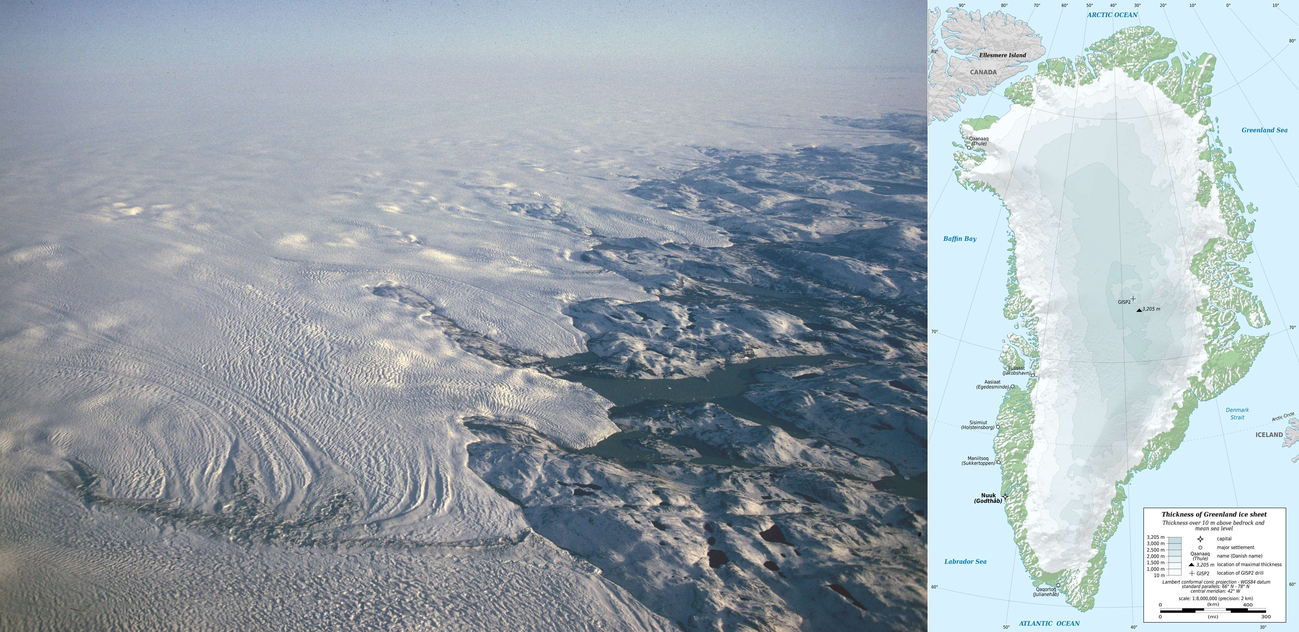
Ice sheets, also called continental glaciers, form across millions of square kilometers of land and are thousands of meters thick. Earth’s largest ice sheets are located on Greenland and Antarctica. The Greenland ice sheet is the largest ice mass in the Northern Hemisphere, with an extensive surface area of over 2 million sq km (1,242,700 sq mi) and an average thickness of up to 1,500 meters (5,000 ft, almost a mile).
The Antarctic ice sheet is even larger and covers almost the entire continent. The thickest parts of the Antarctic ice sheet are over 4,000 meters thick (>13,000 ft or 2.5 mi). Its weight depresses the Antarctic bedrock to below sea level in many places. The cross-sectional diagram comparing the Greenland and Antarctica ice sheets illustrates the size difference between the two.
Ice cap glaciers are smaller versions of ice sheets that cover less than 50,000 km2, usually occupy higher elevations, and may cover tops of mountains. There are several ice caps on Iceland. A small ice cap called Snow Dome is near Mount Olympus on the Olympic Peninsula in the state of Washington.
The figure shows the size of the ancient Laurentide ice sheet in the Northern Hemisphere. This ice sheet was present during the last glacial maximum event, also known as the last ice age.

Take this quiz to check your comprehension of this section.
If you are using an offline version of this text, access the quiz for Section 13.4 via the QR code.
13.5 Glacier Dynamics
13.5.1 Glacier Movement
As the ice accumulates, it begins to flow downward under its own weight. In 1948, glaciologists installed hollow vertical rods in the Jungfraufirn Glacier in the Swiss Alps to measure changes in its movement over two years. This study showed that the ice at the surface was fairly rigid and ice within the glacier was actually flowing downhill. The cross-sectional diagram of an alpine (valley) glacier shows that the rate of ice movement is slow near the bottom and fastest in the middle, with the top ice being carried along on the ice below.
One of the unique properties of ice is that it melts under pressure. About half of the overall glacial movement was from sliding on a film of meltwater along the bedrock surface, with the other half from internal flow. Ice near the surface of the glacier is rigid and brittle to a depth of about 50 m (165 ft). In this brittle zone, large ice cracks called crevasses form on the glacier’s moving surface. These crevasses can be covered and hidden by a snow bridge and are a hazard for glacier travelers.
Below the brittle zone, the pressure typically exceeds 100 kilopascals (kPa), which is approximately 100,000 times atmospheric pressure. Under this applied force, the ice no longer breaks, but rather it bends or flows in a zone called the plastic zone. This plastic zone represents the great majority of glacier ice. The plastic zone contains a fair amount of sediment of various grades from boulders to silt and clay. As the bottom of the glacier slides and grinds across the bedrock surface, these sediments act as grinding agents and create a zone of significant erosion.
13.5.2 Glacial Budget
A glacial budget is like a bank account, with the ice being the existing balance. If there is more income (snow accumulating in winter) than expense (snow and ice melting in summer), then the glacial budget shows growth. A positive or negative balance of ice in the overall glacial budget determines whether a glacier advances or retreats, respectively. The area in which the ice balance grows is called the zone of accumulation. The area where ice balance is shrinking is called the zone of ablation.
The diagram shows these two zones and the equilibrium line. In the zone of accumulation, the snow-accumulation rate exceeds the snow-melting rate and the ice surface is always covered with snow. The equilibrium line, also called the snowline or firnline, marks the boundary between the zones of accumulation and ablation. Below the equilibrium line in the zone of ablation, the melting rate exceeds snow accumulation, leaving the bare ice surface exposed. The position of the firnline changes during the season and from year to year as a reflection of a positive or negative ice balance in the glacial budget. Of the two variables affecting a glacier’s budget, winter accumulation and summer melt, summer melt matters most to a glacier’s budget. Cool summers promote glacial advance, and warm summers promote glacial retreat.
If a handful of warmer summers promote glacial retreat, then global climate warming over decades and centuries will accelerate glacial melting and retreat even faster. Global warming due to human burning of fossil fuels is causing the ice sheets to lose, in years, an amount of mass that would normally take centuries. Current glacial melting is contributing to sea levels rising more quickly than expected based on previous history.
As the Antarctica and Greenland ice sheets melt during global warming, they become thinner or deflate. The edges of the ice sheets break off and fall into the ocean in a process called calving, becoming floating icebergs. A fjord is a steep-walled valley flooded with seawater. The narrow shape of a fjord has been carved out by a glacier during a cooler climate period. During a warming trend, glacial meltwater may raise the sea level in fjords and flood formerly dry valleys. Glacial retreat and deflation are well illustrated in the 2009 TED Talk “Time-lapse proof of extreme ice loss” by James Balog.

Video 13.3: Time-lapse proof of extreme ice loss, by James Balog
If you are using an offline version of this text, access this TED Talk via the QR code.

Take this quiz to check your comprehension of this section.
If you are using an offline version of this text, access the quiz for Section 13.5 via the QR code.
13.6 Glacial Landforms
Both alpine and continental glaciers create two categories of landforms: erosional and depositional. Erosional landforms are formed by the removal of material. Depositional landforms are formed by the addition of material. Because glaciers were first studied by eighteenth- and nineteenth-century geologists in Europe, the terminology applied to glaciers and glacial features contains many terms derived from European languages.
13.6.1 Erosional Glacial Landforms
Erosional landforms are created when moving masses of glacial ice slide and grind over bedrock. Glacial ice contains large amounts of poorly sorted sand, gravel, and boulders that have been plucked and pried from the bedrock. As the glaciers slide across the bedrock, they grind the sediments into a fine powder called rock flour. Rock flour acts as fine grit that polishes the surface of the bedrock to a smooth finish called glacial polish. Larger rock fragments scrape over the surface, creating elongated grooves called glacial striations.
Alpine glaciers produce a variety of unique erosional landforms, such as U-shaped valleys, arêtes, cirques, tarns, horns, cols, hanging valleys, and truncated spurs. In contrast, stream-carved canyons have a V-shaped profile when viewed in cross section. Glacial erosion transforms a former V-shaped stream valley into a U-shaped one. Glaciers are typically wider than streams of similar length, and since glaciers tend to erode both at their bases and their sides, they erode V-shaped valleys into relatively flat-bottomed broad valleys with steep sides and a distinctive U shape. As seen in the images, Little Cottonwood Canyon near Salt Lake City, Utah, was occupied by an ice age glacier that extended down to the mouth of the canyon and into Lake Bonneville. Today, that U-shaped valley hosts many erosional landforms, including polished and striated rock surfaces. In contrast, Big Cottonwood Canyon to the north of Little Cottonwood Canyon has retained the V-shape in its lower portion, indicating that its glacier did not extend clear to its mouth but was confined to its upper portion.

When glaciers carve two U-shaped valleys adjacent to each other, the ridge between them tends to be sharpened into a sawtooth feature called an arête. At the head of a glacially carved valley is a bowl-shaped feature called a cirque. The cirque represents where the head of the glacier eroded the mountain by plucking rock away from it and the weight of the thick ice eroded out a bowl. After the glacier is gone, the bowl at the bottom of the cirque often fills with precipitation and is occupied by a lake called a tarn. When three or more mountain glaciers erode headward at their cirques, they produce horns—steep-sided, spire-shaped mountains. Low points along arêtes or between horns are mountain passes termed cols. Where a smaller tributary glacier flows into a larger trunk glacier, the smaller glacier cuts down less. Once the ice has gone, the tributary valley is left as a hanging valley, sometimes with a waterfall plunging into the main valley. As the trunk glacier straightens and widens a V-shaped valley and as it erodes the ends of side ridges, a steep triangle-shaped cliff is formed called a truncated spur.
13.6.2 Depositional Glacial Landforms
Depositional landforms and materials are produced from deposits left behind by a retreating glacier. All glacial deposits are called drift. These include till, tillites, diamictites, terminal moraines, recessional moraines, lateral moraines, medial moraines, ground moraines, silt, outwash plains, glacial erratics, kettles, kettle lakes, crevasses, eskers, kames, and drumlins.
Glacial ice carries a lot of sediment, which is called till when deposited by a melting glacier. Till is poorly sorted, with grain sizes ranging from clay and silt to pebbles and boulders. These clasts may be striated. Many depositional landforms are composed of till. The term tillite refers to lithified rock having glacial origins. Diamictite refers to a lithified rock that contains a wide range of clast sizes; this includes glacial till but is a more objective and descriptive term for any rock with a wide range of clast sizes.
Moraines are mounded deposits consisting of glacial till carried in the glacial ice and rock fragments dislodged by mass wasting from the U-shaped valley walls. The glacier acts like a conveyor belt, carrying and depositing sediment at the end of and along the sides of theice flow. Because the ice in the glacier always flows downslope, every glacier has moraines built up at its terminus, even if it is not advancing.
Moraines are classified by their location with respect to the glacier. A terminal moraine is a ridge of till located at the end or terminus of the glacier. Recessional moraines are left by retreating glaciers pausing in their retreats. Lateral moraines accumulate along the sides of the glacier from material mass wasted from the valley walls. When two tributary glaciers merge, the two lateral moraines combine to form a medial moraine running down the center of the combined glacier. Ground moraine is a veneer of till left on the land as the glacier melts.
In addition to moraines, glaciers leave behind other depositional landforms. Silt, sand, and gravel produced by the intense grinding process are carried by streams of water and deposited in front of the glacier in an area called the outwash plain. Retreating glaciers may leave behind large boulders that don’t match the local bedrock. These are called glacial erratics. When continental glaciers retreat, they can leave behind large blocks of ice within the till. These ice blocks melt and create a depression in the till called a kettle. If the depression later fills with water, it is called a kettle lake.
If meltwater flowing over the ice surface descends into crevasses in the ice, it may find a channel and continue to flow in sinuous channels within or at the base of the glacier. Within or under continental glaciers, these streams carry sediments. When the ice recedes, the accumulated sediment is deposited as a long sinuous ridge known as an esker. Meltwater descending down through the ice or over the margins of the ice may deposit mounds of till in hills called kames.
Drumlins are common in continental glacial areas of Germany, New York, and Wisconsin, where they are typically found in fields with great numbers. A drumlin is an elongated, asymmetrical teardrop-shaped hill reflecting ice movement with its steepest side pointing upstream to the flow of ice and its streamlined, low-angled side pointing downstream in the direction of ice movement.
Glacial scientists debate the origins of drumlins. A leading idea is that drumlins are created from accumulated till being compressed and sculpted under a glacier that retreated then advanced again over its own ground moraine. Another idea is that meltwater catastrophically flooded under the glacier and carved the till into these streamlined mounds. Still another proposes that the weight of the overlying ice statically deformed the underlying till.

Complete this interactive activity to check your understanding.
If you are using an offline version of this text, access this interactive activity via the QR code.
13.6.3 Glacial Lakes
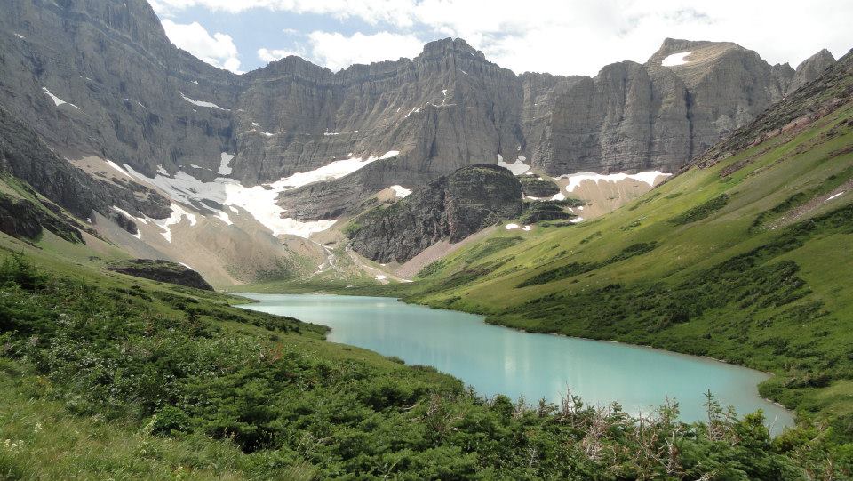
Glacial lakes are commonly found in alpine environments. A lake confined within a glacial cirque is called a tarn. A tarn forms when the depression in the cirque fills with precipitation after the ice is gone. Examples of tarns include Silver Lake near Brighton ski resort in Big Cottonwood Canyon, Utah, and Avalanche Lake in Glacier National Park, Montana.
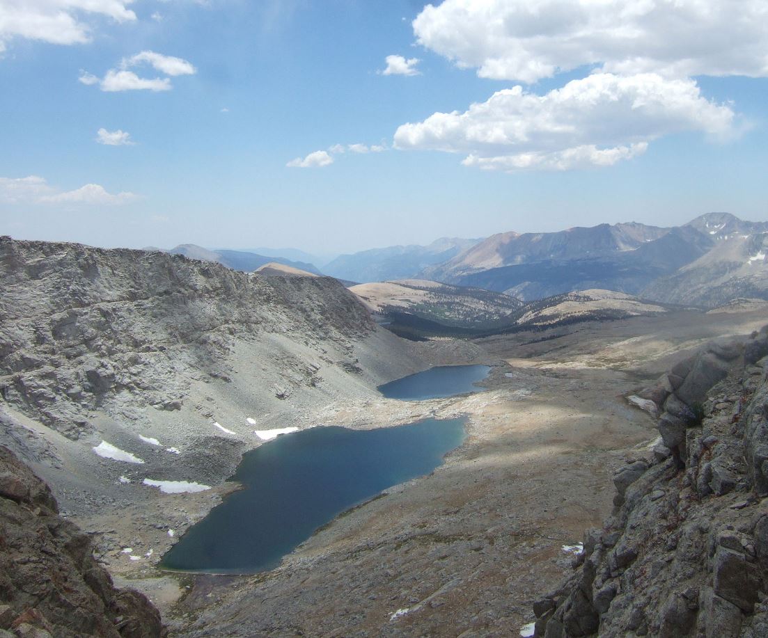
When recessional moraines create a series of isolated basins in a glaciated valley, the resulting chain of lakes is called paternoster lakes. Lakes filled by glacial meltwater often look milky due to finely ground material called rock flour suspended in the water.
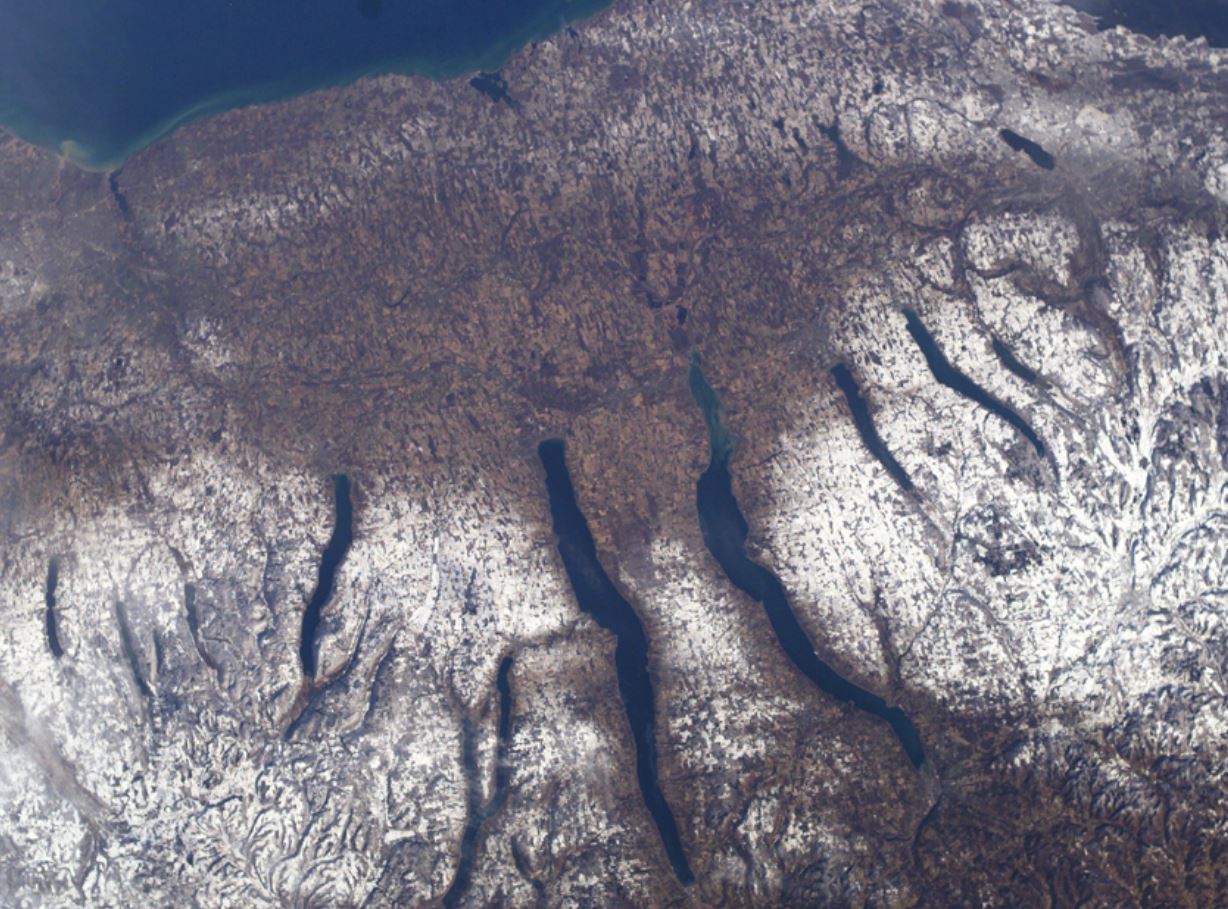
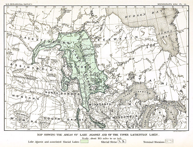
Long, glacially carved depressions filled with water are known as finger lakes. Proglacial lakes form along the edges of all the largest continental ice sheets, such as Antarctica and Greenland. The crust is depressed isostatically by the overlying ice sheet, and these basins fill with glacial meltwater. Many such lakes, some of them huge, existed at various times along the southern edge of the Laurentide ice sheet. Lake Agassiz, Manitoba, Canada, is a classic example of a proglacial lake. Lake Winnipeg serves as the remnant of a much larger proglacial lake.
Other proglacial lakes were formed when glaciers dammed rivers and flooded the river valley. A classic example is Lake Missoula, which formed when a lobe of the Laurentide ice sheet blocked the Clark Fork River about 18,000 years ago. Over about 2,000 years, the ice dam holding back Lake Missoula failed several times. During each breach, the lake emptied across parts of eastern Washington, Oregon, and Idaho into the Columbia River Valley and eventually the Pacific Ocean. After each breach, the dam reformed and the lake refilled. Each breach produced a catastrophic flood over a few days. Scientists estimate that this cycle of ice dam, proglacial lake, and torrential massive flooding happened at least 25 times over a span of 20 centuries. The rate of each outflow is believed to have equaled the combined discharge of all of Earth’s current rivers combined.
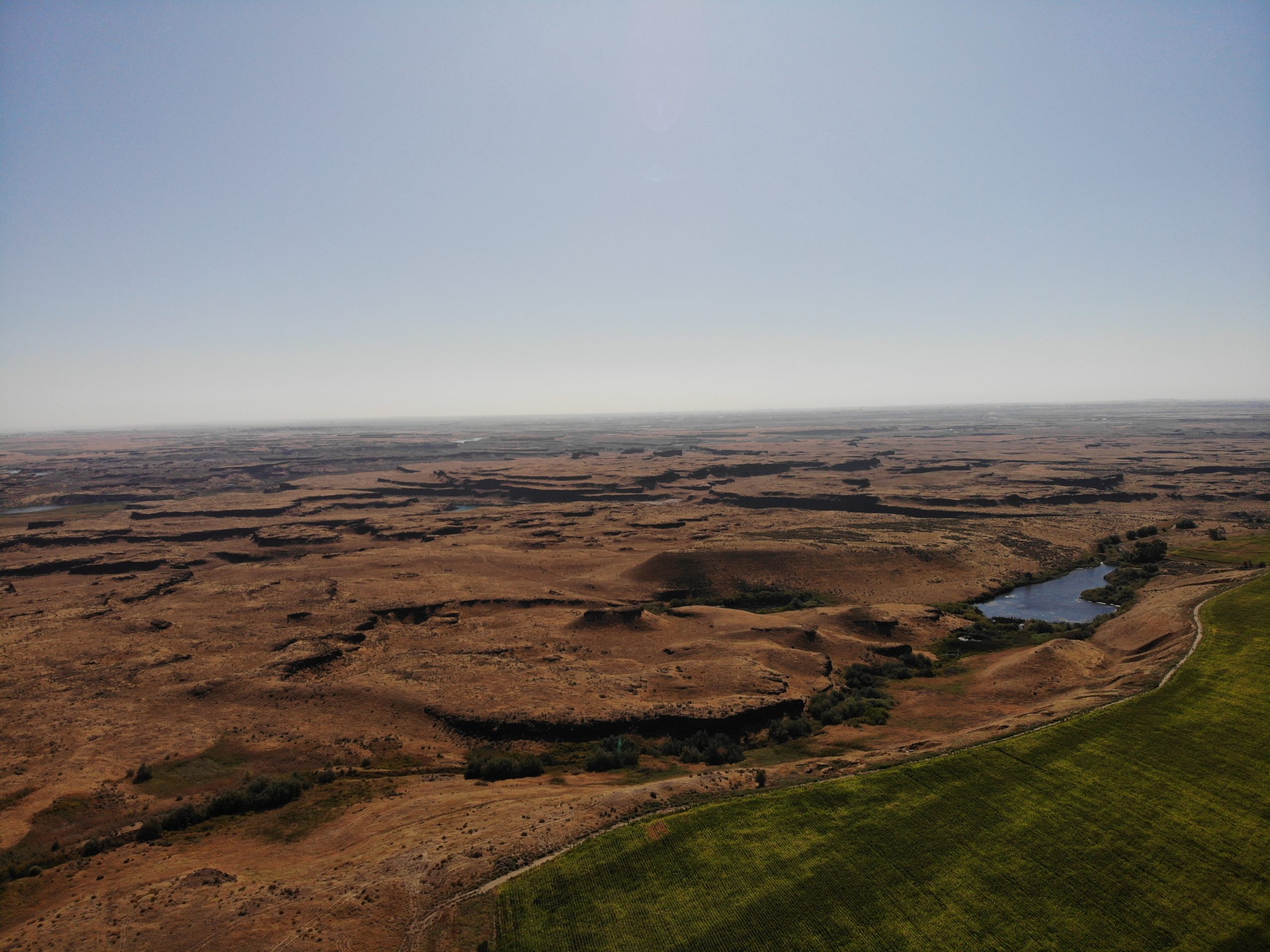
The landscape produced by these massive floods is preserved in the Channeled Scablands of Idaho, Washington, and Oregon.
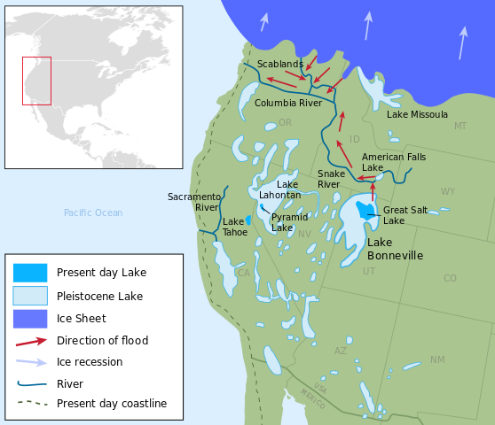
Pluvial lakes form in humid environments that experience low temperatures and high precipitation. During the last glaciation, the climate of most of the Western United States was cooler and more humid than today. Under these low-evaporation conditions, many large lakes, called pluvial lakes, formed in the basins of the Basin and Range Province. Two of the largest were Lake Bonneville and Lake Lahontan. Lake Lahontan was in northwestern Nevada, while Bonneville occupied much of western Utah and eastern Nevada. Figure 13.58 illustrates the tremendous size of Lake Bonneville. The lake level fluctuated greatly over the centuries, leaving several pronounced old shorelines marked by wave-cut terraces. These old shorelines can be seen on mountain slopes throughout the western portion of Utah, including the Salt Lake Valley, indicating that the now heavily urbanized valley was once filled with hundreds of feet of water. Lake Bonneville’s level peaked around 18,000 years ago when a breach occurred at Red Rock Pass in Idaho and water spilled into the Snake River. The flooding rapidly lowered the lake level and scoured the Idaho landscape across the Pocatello Valley, the Snake River Plain, and Twin Falls. The floodwaters ultimately flowed into the Columbia River across part of the scablands area at an incredible discharge rate of about 4,750 cu km/sec (1,140 cumi/sec).
For comparison, this discharge rate would drain the volume of Lake Michigan completely dry within a few days.
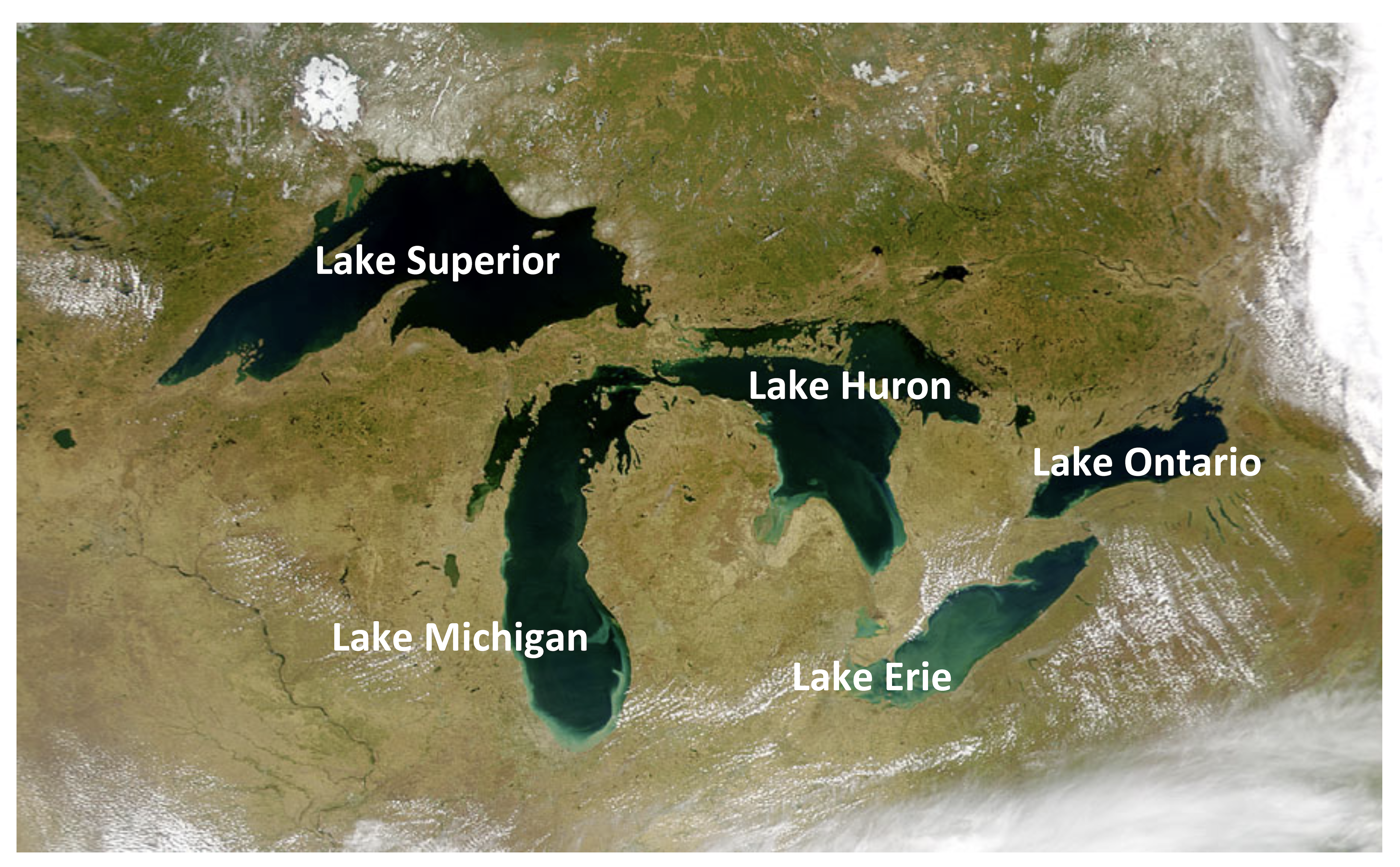
The five Great Lakes in North America’s Upper Midwest are proglacial lakes that originated during the last ice age. The lake basins were originally carved by the encroaching continental ice sheet. The basins were later exposed as the ice retreated about 14,000 years ago and were then filled by precipitation.

Take this quiz to check your comprehension of this section.
If you are using an offline version of this text, access the quiz for Section 13.6 via the QR code.
13.7 Ice Age Glaciations
A glaciation (or ice age) occurs when the Earth’s climate becomes cold enough that continental ice sheets expand, covering large areas of land. Four major, well-documented ]glaciations have occurred in Earth’s history: one during the Archean-early Proterozoic Eon, ~2.5 billion years ago; another in late Proterozoic Eon, ~700 million years ago; another in the Pennsylvanian, 323 to 300 million years ago; and most recently during the Pliocene-Pleistocene epochs, starting 2.5 million years ago (Chapter 8). Some scientists also recognize a minor glaciation around 440 million years ago in Africa.
The best-studied glaciation is, of course, the most recent. This infographic illustrates the glacial and climate changes over the last 20,000 years, ending with those caused by human actions since the Industrial Revolution. The Pliocene-Pleistocene glaciation was a series of several glacial cycles, possibly 18 in total. Antarctic ice-core records exhibit especially strong evidence for eight glacial advances occurring within the last 420,000 years. The last of these is known in popular media as “The Ice Age,” but geologists refer to it as the Last Glacial Maximum. The glacial advance reached its maximum between 26,500 and 19,000 years ago.
13.7.1 Causes of Glaciations
Glaciations occur due to both long-term and short-term factors. In the geologic sense, long-term means a scale of tens to hundreds of millions of years and short-term means a scale of hundreds to thousands of years.
Long-term causes include plate tectonics breaking up the supercontinents (see Wilson cycle, Chapter 2), moving land masses to high latitudes near the North or South Poles and changing ocean circulation. For example, the closing of the Panama Strait and isolation of the Pacific and Atlantic Oceans may have triggered a change in precipitation cycles, which combined with a cooling climate to help expand the ice sheets.
Short-term causes of glacial fluctuations are attributed to the cycles in the Earth’s rotational axis and to variations in the Earth’s orbit around the Sun that affect the distance between Earth and the Sun. Called Milankovitch cycles, these cycles affect the amount of incoming solar radiation, causing short-term cycles of warming and cooling.
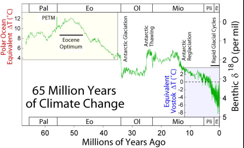
During the Cenozoic Era, carbon dioxide levels steadily decreased from a maximum in the Paleocene, causing the climate to gradually cool. By the Pliocene, ice sheets began to form. The effects of the Milankovitch cycles created short-term cycles of warming and cooling within the larger glaciation event.
Milankovitch cycles are three orbital changes named after the Serbian astronomer Milutan Milankovitch. The three orbital changes are called precession, obliquity, and eccentricity. Precession is the wobbling of Earth’s axis with a period of about 21,000 years; obliquity is changes in the angle of Earth’s axis with a period of about 41,000 years; and eccentricity is variations in the Earth’s orbit around the Sun leading to changes in distance from the Sun with a period of 93,000 years. These orbital changes created a 41,000-year-long glacial-interglacial Milankovitch cycle from 2.5 to 1 million years ago, followed by another longer cycle of about 100,000 years from 1 million years ago to today (see the Wikipedia page on Milankovitch cycles).

Complete this interactive activity to check your understanding.
If you are using an offline version of this text, access this interactive activity via the QR code.
Watch the video to see summaries of the ice ages, including their characteristics and causes.

Video 13.4: Ice ages and climate cycles
If you are using an offline version of this text, access this YouTube video via the QR code.
13.7.2 Sea-Level Change and Isostatic Rebound
When glaciers melt and retreat, two things happen: water runs off into the ocean, causing sea levels to rise worldwide, and the land, released from its heavy covering of ice, rises due to isostatic rebound. Since the Last Glacial Maximum about 19,000 years ago, sea level has risen about 125 m (400 ft). A global change in sea level is called eustatic sea-level change. During a warming trend, sea level rises due to more water being added to the ocean and also because of thermal expansion of seawater. About half of the Earth’s eustatic sea level rise during the last century has been the result of glaciers melting and about half due to thermal expansion. Thermal expansion describes how a solid, liquid, or gas expands in volume with an increase in temperature. This 30-second video demonstrates thermal expansion with the classic brass ball and ring experiment.

Video 13.5: Thermal expansion
If you are using an offline version of this text, access this YouTube video via the QR code.
Relative sea-level change includes vertical movement of both eustatic sea level and continents on tectonic plates. In other words, sea-level change is measured relative to land elevation. For example, if the land rises a lot and sea level rises only a little, then the relative sea level would appear to drop.
Continents sitting on the lithosphere can move vertically upward as a result of two main processes, tectonic uplift and isostatic rebound. Tectonic uplift occurs when tectonic plates collide (see Chapter 2). Isostatic rebound describes the upward movement of lithospheric crust sitting on top of the asthenospheric layer below it. Continental crust bearing the weight of continental ice sinks into the asthenosphere, displacing it. After the ice sheet melts away, the asthenosphere flows back in and continental crust floats back upward. Erosion can also create isostatic rebound by removing large masses like mountains and transporting the sediment away (think of the Mesozoic removal of the Alleghanian Mountains and the uplift of the Appalachian Plateau; Chapter 8), albeit this process occurs more slowly than relatively rapid glacier melting.

The isostatic-rebound map in Figure 13.61 shows rates of vertical crustal movement worldwide. The highest rebound rate is indicated by the blue-to-purple zones (top end of the scale). The orange-to-red zones (bottom end of the scale) surrounding the high-rebound zones indicate isostatic lowering as adjustments in displaced subcrustal material have taken place.
Most glacial isostatic rebound occurs where continental ice sheets rapidly melted about 19,000 years ago, such as in Canada and Scandinavia. Its effects can be seen wherever ice age ice or water bodies are or were present on continental surfaces and in terraces on river floodplains that cross these areas. Isostatic rebound occurred in Utah when the water from Lake Bonneville drained away. North America’s Great Lakes also exhibit emergent coastline features caused by isostatic rebound since the continental ice sheet retreated.

Take this quiz to check your comprehension of this section.
If you are using an offline version of this text, access the quiz for Section 13.7 via the QR code.
Summary
Approximately 30% of Earth’s surface is arid lands shaped by factors such as latitude, atmospheric circulation, and terrain. Deserts between 15° and 30° latitude are formed by descending air masses in the atmosphere’s major cells, including the Sahara and deserts of the Middle East. Other deserts, like those in western North America and the Atacama in South America, form in rain shadows behind mountain ranges. Dry, descending air also creates polar deserts at the poles.
Atmospheric circulation, involving the Hadley, Ferrel, and polar cells, drives desert formation. Warm air rises in the tropics, dries out, and descends in the arid zones of both hemispheres. The Earth’s rotation deflects air masses, producing prevailing winds like the trade winds and westerlies. Complex interactions of latitude, rain shadows, and ocean currents make the Atacama Desert the driest place on Earth.
In deserts, weathering occurs slowly due to low moisture, with unique features like desert varnish and wind-driven erosion. Wind transports sand, shaping landforms like dunes and eroded bedrock features. Poor land management can accelerate desertification, a global problem that degrades once-productive land into desert.
Glaciers form when snowfall exceeds melting, compressing snow into ice. They can be classified into alpine glaciers in valleys, ice sheets covering continents, and ice caps over smaller areas at high elevations. As glaciers grow, they flow under their own weight, with the upper brittle ice cracking into crevasses, while the lower plastic zone bends and flows. Rock debris, known as moraine, gets carried along, grinding against bedrock and causing significant erosion.
Glaciers have a budget that balances accumulation and ablation. If more ice accumulates than melts, the glacier advances; if melting exceeds accumulation, the glacier recedes, a trend seen globally due to warming. Glaciers shape landscapes by carving U-shaped valleys and depositing features like moraines, drumlins, and kettle lakes. Their meltwater forms outwash plains and can create massive floods, as seen with ice age lakes like Lake Missoula, which caused widespread erosion in areas like the Channeled Scablands.

Take this quiz to check your comprehension of this chapter.
If you are using an offline version of this text, access the quiz for Chapter 13 via the QR code.
Text References
- Allen, P.A., and Etienne, J.L. (2008). Sedimentary challenge to snowball Earth. Nat. Geosci., 1(12), 817–825.
- Bagnold, R. A. (1941). The physics of blown sand and desert dunes: Methum, 265.
- Berner, R.A. (1998). The carbon cycle and carbon dioxide over Phanerozoic time: The role of land plants. Philos. Trans. R. Soc. Lond. B Biol. Sci., 353(1365), 75–82.
- Boggs, S. (2006). Principles of sedimentology and stratigraphy: Pearson Prentice Hall. http://agris.fao.org/agrissearch/search.do?recordID=US201300110702.
- Clements, T. (1952). Wind-blown rocks and trails on Little Bonnie Claire Playa, Nye County, Nevada. Journal of Sedimentary Research, 22(3). Society for Sedimentary Geology. http://archives.datapages.com/data/sepm/journals/v01-32/data/022/022003/0182.htm.
- Collado, G.A., Valladares, M.A., and Méndez, M.A. (2013). Hidden diversity in spring snails from the Andean Altiplano, the second highest plateau on Earth, and the Atacama Desert, the driest place in the world. Zoological Studies, 52(1), 50.
- Cunningham, W.L., Leventer, A., Andrews, J.T., Jennings, A.E., and Licht, K.J. (1999). Late Pleistocene–Holocene marine conditions in the Ross Sea, Antarctica: Evidence from the diatom record. The Holocene, 9(2), 129–139.
- Deynoux, M., Miller, J.M.G., and Domack, E.W. (2004). Earth’s glacial record: World and regional geology: Cambridge University Press, World and Regional Geology.
- Earle, S. (2015). Physical geology OER textbook: BC Campus OpenEd.
- Easterbrook, D.J. (1999). Surface processes and landforms: Pearson College Division.
- Eyles, N., and Januszczak, N. (2004). “Zipper-rift”: A tectonic model for Neoproterozoic glaciations during the breakup of Rodinia after 750 Ma. Earth-Sci. Rev. 65(1–2), 1–73.
- Francey, R.J., Allison, C.E., Etheridge, D.M., Trudinger, C.M., et al. (1999). A 1000-year high precision record of δ13C in atmospheric CO2. Tellus B Chem. Phys. Meteorol.
- Geist, H. (2005). The causes and progression of desertification: Ashgate Aldershot.
- Grayson, D.K. (1993). The desert’s past: A natural prehistory of the Great Basin: Smithsonian Institute Press.
- Gutro, R. (2005). NASA – What’s the difference between weather and climate? Online, http://www.nasa.gov/mission_pages/noaa-n/climate/climate_weather.html, accessed September 2016.
- Hadley, G. (1735). Concerning the cause of the general trade-winds: Philosophical Transactions, 39(436-444). The Royal Society, 58–62.
- Hartley, A.J., and Chong, G. (2002). Late Pliocene age for the Atacama Desert: Implications for the Desertification of Western South America. Geology, 30(1), 43–46. http://geology.gsapubs.org.
- Hedin, S.A. (1903). Central Asia and Tibet. Vol. 1: Hurst and Blackett, limited.
- Hoffman, P.F., Kaufman, A.J., Halverson, G.P., and Schrag, D.P. (1998). A neoproterozoic snowball Earth. Science, 281(5381), 1342–1346.
- Hooke, R.L. (1967). Processes on arid-region alluvial fans. The Journal of Geology, 75(4), 438–60.
- King, L.C. (1953). Canons of landscape evolution. Geological Society of America Bulletin 64(7), 721–52.
- Kletetschka, G., Hooke, R.L., Ryan, A., Fercana, G., McKinney, E. and Schwebler, K.P. (2013). Sliding stones of Racetrack Playa, Death Valley, USA: The roles of rock thermal conductivity and fluctuating water levels. Geomorphology, 195(August), 110–17.
- Kopp, R.E., Kirschvink, J.L., Hilburn, I.A., and Nash, C.Z. (2005). The Paleoproterozoic snowball Earth: A climate disaster triggered by the evolution of oxygenic photosynthesis. Proc. Natl. Acad. Sci. U.S.A., 102(32), 11131–11136.
- Laity, J.E. (2009). Landforms, landscapes, and processes of aeolian erosion, in Geomorphology of desert environments, (Parsons, A.J., and Abrahams, A.D., eds.): Springer Netherlands, 597–627.
- Lean, J., Beer, J., and Bradley, R. (1995). Reconstruction of solar irradiance since 1610: Implications for climate change. Geophys. Res. Lett., 22(23), 3195–3198.
- Levitus, S., Antonov, J.I., Wang, J., Delworth, T.L., Dixon, K.W., and Broccoli, A.J. (2001). Anthropogenic warming of Earth’s climate system. Science, 292(5515), 267–270.
- Lindsey, R. (2009). Climate and Earth’s energy budget: Feature articles. NASA. Online, http://earthobservatory.nasa.gov, accessed September 2016.
- Littell, E., and Littell, R.S. (1846). Littell’s living age: T.H. Carter & Company.
- Livingstone, I., and Warren, A. (1996). Aeolian geomorphology: An introduction: Longman.
- Muhs, D.R., and Bettis, E.A. (2003). Quaternary Loess-Paleosol Sequences as Examples of Climate-Driven Sedimentary Extremes.” Special Papers-Geological Society of America. Boulder, Colo.; Geological Society of America; 1999, 53–74.
- Norris, R.D., Norris, J.M., Lorenz, R.D., Ray, J., and Jackson, B. (2014). Sliding rocks on Racetrack Playa, Death Valley National Park: First observation of rocks in motion. PloS One, 9(8), e105948. http://journals.plos.org.
- North Carolina State University (2013a). Composition of the atmosphere.
- North Carolina State University (2013b). Composition of the atmosphere. Online, http://climate.ncsu.edu/edu/k12/.AtmComposition, accessed September 2016.
- Oreskes, N. (2004). The scientific consensus on climate change. Science, 306(5702), 1686–1686.
- Pachauri, R.K., Allen, M.R., Barros, V.R., Broome, J., Cramer, W., Christ, R., Church, J.A., Clarke, L., Dahe, Q., Dasgupta, P., Dubash, N.K., Edenhofer, O., Elgizouli, I., Field, C.B., et al. (2014). Climate change 2014: Synthesis report. Contribution of Working Groups I, II and III to the Fifth Assessment Report of the Intergovernmental Panel on Climate Change (R. K. Pachauri & L. Meyer, eds.): Geneva, Switzerland, IPCC.
- Santer, B.D., Mears, C., Wentz, F.J., Taylor, K.E., Gleckler, P.J., Wigley, T.M.L., Barnett, T.P., Boyle, J.S., Brüggemann, W., Gillett, N.P., Klein, S.A., Meehl, G.A., Nozawa, T., Pierce, D.W., et al. (2007). Identification of human-induced changes in atmospheric moisture content. Proc. Natl. Acad. Sci. U.S.A., 104(39), 15248–15253.
- Schopf, J.W., and Klein, C. (1992). Late-Proterozoic low-latitude global glaciation: The snowball Earth, in Schopf, J.W., and Klein, C. (eds.). The Proterozoic biosphere: A multidisciplinary study: Cambridge University Press, p. 51–52.
- Shao, Y. (2008). Physics and modelling of wind erosion: Springer Science & Business Media.
- Stanley, G.M. (1955). Origin of playa stone tracks, racetrack playa, Inyo County, California. Geological Society of America Bulletin, 66(11), 1329–50. http://gsabulletin.gsapubs.org.
- Walker, A.S. (1996). Deserts: Geology and resources: U.S. Government Printing Office. https://pubs.er.usgs.gov/publication/7000004.
- Webb, T., and Thompson, W. (1986). Is vegetation in equilibrium with climate? How to interpret late-Quaternary pollen data. Vegetatio, 67(2), 75–91.
- Weissert, H. (2000). Deciphering methane’s fingerprint. Nature, 406(6794), 356–357.
- Whitlock, C., and Bartlein, P.J. (1997). Vegetation and climate change in northwest America during the past 125 kyr. Nature, 388(6637), 57–61.
- Wilson, I.G. (1971). Desert sandflow basins and a model for the development of ergs. The Geographical Journal, 137(2), 180–99.
- Wolpert, S. (2009). New NASA temperature maps provide a ‘whole new way of seeing the moon’. Online, http://newsroom. ucla.edu/releases/new-nasa-temperature-maps-provide-102070, accessed February 2017.
- Zachos, J., Pagani, M., Sloan, L., Thomas, E., and Billups, K. (2001). Trends, rhythms, and aberrations in global climate. 65 Ma to present. Science, 292(5517), 686–693.
Figure References
Figure 13.1: World hot deserts (Koppen BWh). M.C. Peel, B.L. Finlayson, and T.A. McMahon; adapted by Me ne frego. 2011. CC BY-SA 3.0. https://en.wikipedia.org/wiki/File:Koppen_World_Map_BWh.png
Figure 13.2: Mountainous areas in front of the prevailing winds create a rain shadow. domdomegg. 2015. CC BY 4.0. https://commons.wikimedia.org/wiki/File:Rainshadow_copy.svg
Figure 13.3: In this image from the ISS, the Sierra Nevada Mountains are perpendicular to prevailing westerly winds, creating a rain shadow to the east (bottom of the image). NASA. 2003. Public domain. https://earthobservatory.nasa.gov/images/3273/southern-sierra-nevada-and-owens-lake
Figure 13.4: Generalized atmospheric circulation. NASA. 2009. Public domain. https://commons.wikimedia.org/wiki/File:Earth_Global_Circulation.jpg
Figure 13.5: USGS map of the Great Basin Desert. United States Geological Survey (USGS). 2012. Public domain. https://commons.wikimedia.org/wiki/File:Central_Basin_and_Range_ecoregion.gif
Figure 13.6: Map of the Atacama Desert (yellow) and surrounding related climate areas (orange). cobaltcigs. 2010. CC BY-SA 3.0. https://en.wikipedia.org/wiki/File:Atacama_map.svg
Figure 13.7: The polar vortex of mid-November, 2013. National Oceanic and Atmospheric Administration (NOAA). 2014. Public domain. https://commons.wikimedia.org/wiki/File:November2013_polar_vortex_geopotentialheight_mean_Large.jpg
Figure 13.8: In the inertial frame of reference of the top picture, the ball moves in a straight line. Hubi. 2003. CC BY-SA 3.0. https://commons.wikimedia.org/wiki/File:Corioliskraftanimation.gif
Figure 13.9: Forces acting on a mass moving east–west on the rotating Earth that produce the Coriolis effect. Kindred Grey. 2022. CC BY 4.0.
Figure 13.10: Inertia of air masses caused by the Coriolis effect in the absence of other forces. Kes47. 2015. CC BY-SA 3.0. https://commons.wikimedia.org/wiki/File:Coriolis_effect.svg
Figure 13.11: Gyres of the Earth’s oceans. Canuckguy; adapted by Shadowxfox and Popadius. 2012. Public domain. https://commons.wikimedia.org/wiki/File:Corrientes-oceanicas-en.svg
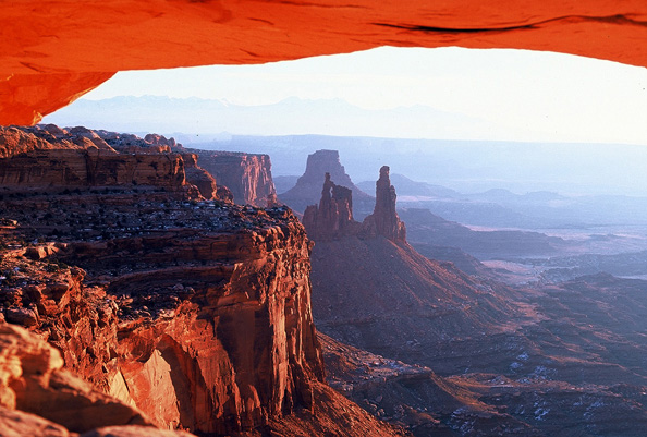
Figure 13.12: Weathering and erosion of Canyonlands National Park has created a unique landscape that includes arches, cliffs, and spires. Rick. 2005. CC BY 2.0. https://commons.wikimedia.org/wiki/File:Mesa_Arch_Canyonlands_National_Park.jpg
Figure 13.13: Newspaper Rock, located in Petrified Forest National Park, is a site with many petroglyphs carved into desert varnish. Laura Neser. March 2022. CC BY-NC.
Figure 13.14: A dust storm (haboob) hits Texas in 2019. Jakeorin. 2019. CC BY-SA 4.0. https://commons.wikimedia.org/wiki/File:Haboob_in_Big_Spring,_TX.jpg
Figure 13.15: Diagram showing the mechanics of saltation. NASA. 2002. Public domain. https://commons.wikimedia.org/wiki/File:Saltation-mechanics.gif
Figure 13.16: Enlarged image of frosted and rounded windblown sand grains. Wilson44691. 2008. Public domain. https://commons.wikimedia.org/wiki/File:CoralPinkSandDunesSand.jpg
Figure 13.17: A sailing stone at Racetrack Playa in Death Valley National Park, California. Lgcharlot. 2006. CC BY-SA 4.0. https://commons.wikimedia.org/wiki/File:Racetrack_Playa_in_Death_Valley_National_Park.jpg
Figure 13.18: (Top) A yardang near Meadow, Texas. (Bottom) Blowout near Earth, Texas. Yardang: United States Department of Agriculture. 2000. Public domain. https://commons.wikimedia.org/wiki/File:Yardang_Lea-Yoakum_Dunes.jpg, Blowout: Leaflet. 1996. CC BY-SA 3.0. https://commons.wikimedia.org/wiki/File:Blowout_Earth_TX.jpg
Figure 13.19: Wind-carved ventifact in White Desert National Park, Egypt. Christine Schultz. 2003. Public domain. https://commons.wikimedia.org/wiki/File:Weisse_W%C3%BCste.jpg
Figure 13.20: Aerial image of alluvial fan in Death Valley. USGS. 2005. Public domain. https://commons.wikimedia.org/wiki/File:Alluvial_Fan.jpg
Figure 13.21: Bajada along Frisco Peak in Utah. GerthMichael. 2010. CC BY-SA 3.0. https://commons.wikimedia.org/wiki/File:FriscoMountainUT.jpg
Figure 13.22: Inselbergs in the Western Sahara. Nick Brooks. 2007. CC BY 2.0. https://commons.wikimedia.org/wiki/File:Breast-Shaped_Hill.jpg
Figure 13.23: Satellite image of desert playa surrounded by mountains. Robert Simmon, using Landsat data from the USGS and NASA. 2013. Public domain. https://earthobservatory.nasa.gov/images/80913/eye-exam-for-a-satellite
Figure 13.24: (Top) Dry wash (or ephemeral stream). (Bottom) Flash flood in a (different) dry wash. Top: Finetooth. 2010. CC BY-SA 3.0. https://commons.wikimedia.org/wiki/File:Dry_Wash_in_PEFO_NP.jpg Bottom: USGS. 2016. Public domain. https://www.usgs.gov/media/images/a-flooded-river-australia
Figure 13.25: Antelope Canyon is a slot canyon in Arizona formed by the erosion of Navajo Sandstone. It is susceptible to flash flooding, even from rain falling miles away. Laura Neser. March 2022. CC BY-NC.
Figure 13.26: A sand sea or erg in the Sahara Desert. Wsx. 2004. CC BY-SA 3.0. https://commons.wikimedia.org/wiki/File:Sahara_Desert_in_Jalu,_Libya.jpeg
Figure 13.27: Formation of cross-bedding in sand dunes. David Tarailo, GSA, GeoCorps Program. 2015. Public domain. https://commons.wikimedia.org/wiki/File:Formation_of_cross-bedding.jpg
Figure 13.28: Cross-beds in the Navajo Sandstone at Zion National Park. Laura Neser. March 2022. CC BY-NC.
Figure 13.29: NASA image of barchan dune field in coastal Brazil. NASA. 2003. Public domain. https://earthobservatory.nasa.gov/images/3889/coastal-dunes-brazil
Figure 13.30: Satellite image of longitudinal dunes in Egypt. NASA. 2012. Public domain. https://earthobservatory.nasa.gov/images/78151/linear-dunes-great-sand-sea-egypt
Figure 13.31: Parabolic dunes. Po ke jung. 2011. CC BY 3.0. https://commons.wikimedia.org/wiki/File:Parabolic_dune.jpg
Figure 13.32: Star dune in Namib Desert. Dave Curtis. 2005. CC BY-NC-ND 2.0. https://flic.kr/p/4N5Fa
Figure 13.33: The Great Basin. Kmusser; adapted by Hike395. 2022. CC BY-SA 3.0. https://commons.wikimedia.org/wiki/File:Great_Basin_map.gif
Figure 13.34: Typical Basin and Range scene. Matt Affolter (QFL247). 2010. CC BY-SA 3.0. https://commons.wikimedia.org/wiki/File:RidgecrestCA.jpg
Figure 13.35: World map showing desertification vulnerability. USDA. 1998. Public domain. https://commons.wikimedia.org/wiki/File:Desertification_map.png
Figure 13.36: Glacier in the Bernese Alps. Dirk Beyer. 2005. CC BY-SA 3.0. https://commons.wikimedia.org/wiki/File:Grosser_Aletschgletscher_3178.jpg
Figure 13.37: Alpine glaciers of the Alps visible from an airplane en route from Milan, Italy, to Munich, Germany. Laura Neser. September 2023. CC BY-NC.
Figure 13.38: (Left) Greenland ice sheet. (Right) Map showing the thickness of the Greenland ice sheet in meters. Left: Greenland ice sheet. Hannes Grobe. 1995. CC BY-SA 2.5. https://commons.wikimedia.org/wiki/File:Greenland-ice_sheet_hg.jpg. Right: Eric Gaba. 2011. CC BY-SA 3.0. https://commons.wikimedia.org/wiki/File:Greenland_ice_sheet_AMSL_thickness_map-en.svg
Figure 13.39: Cross-sectional view of both Greenland and Antarctic ice sheets drawn to scale for size comparison. Kindred Grey. 2022. CC BY 4.0. Adapted from Steve Earle (CC BY 4.0). https://opengeology.org/textbook/14-glaciers/14-2_steve-earle_antarctic-greenland-2-300×128
Figure 13.40: Snow Dome ice cap near Mount Olympus, Washington (left), and Vatnajökull ice cap in Iceland (right). Left: Mount Olympus Washington by United States National Park Service. 2004. Public domain. https://commons.wikimedia.org/wiki/File:Mount_Olympus_Washington.jpg. Right: Vatnajökull by NASA. 2004. Public domain. https://commons.wikimedia.org/wiki/File:Vatnaj%C3%B6kull.jpeg
Figure 13.41: Maximum extent of Laurentide ice sheet. USGS. 2005. Public domain. https://commons.wikimedia.org/wiki/File:Pleistocene_north_ice_map.jpg
Figure 13.42: Glacial crevasses (left) and cravasse on the Easton Glacier in the North Cascades (right). chevron crevasse by Bethan Davies, 2015 (CC BY-NC-SA 3.0, https://www.antarcticglaciers.org/glacier-processes/structural-glaciology/chevron-crevasse). Glaciereaston by Mauri S. Pelto, 2005 (Public domain, https://en.wikipedia.org/wiki/File:Glaciereaston.jpg).
Figure 13.43: Cross section of a valley glacier showing stress (red numbers) increase with depth under the ice. Kindred Grey. 2022. CC BY 4.0. Adapted from Steve Earle (CC BY 4.0). https://opengeology.org/textbook/14-glaciers/14-2_steve-earle_ice-flow-and-stress
Figure 13.44: Cross-sectional view of an alpine glacier showing internal flow lines, zone of accumulation, snow line, and zone of melting. Kindred Grey. 2022. CC BY 4.0. Adapted from Steven Earle (CC BY 4.0). https://opentextbc.ca/geology/chapter/16-2-how-glaciers-work
Figure 13.45: Fjord. Frédéric de Goldschmidt. 2007. CC BY-SA 3.0. https://sco.wikipedia.org/wiki/File:Geirangerfjord_(6-2007).jpg
Figure 13.46: Glacial striations on granite in Whistler, Canada (left), and glacial striations in Mount Rainier National Park (right). Glacial striations by Amezcackle, 2003 (Public domain, https://en.m.wikipedia.org/wiki/File:Glacial_striations.jpg). Glacial striation 21149 by Walter Siegmund, 2007 (CC BY-SA 3.0, https://commons.wikimedia.org/wiki/File:Glacial_striation_21149.jpg).
Figure 13.47: The U-shape of the Little Cottonwood Canyon, Utah, as it enters into the Salt Lake Valley. Wilson44691. 2008. Public domain. https://commons.wikimedia.org/wiki/File:UshapedValleyUT.jpg
Figure 13.48: Formation of a glacial valley. Cecilia Bernal. 2015. CC BY-SA 4.0. https://commons.wikimedia.org/wiki/File:Glacier_Valley_formation-_Formaci%C3%B3n_Valle_glaciar.gif
Figure 13.49: Cirque with Upper Thornton Lake in the North Cascades National Park, Washington (left). Thornton Lakes 25929 by Walter Siegmund, 2007 (CC BY-SA 3.0, https://commons.wikimedia.org/wiki/File:Thornton_Lakes_25929.jpg). Kinnerly Peak by USGS, 1982 (Public domain, https://uk.wikipedia.org/wiki/%D0%A4%D0%B0%D0%B9%D0%BB:Kinnerly_Peak.jpg). Closeup of Bridalveil Fall seen from Tunnel View in Yosemite NP by Daniel Mayer, 2003 (CC BY-SA 1.0, https://commons.wikimedia.org/wiki/File:Closeup_of_Bridalveil_Fall_seen_from_Tunnel_View_in_Yosemite_NP.jpg).
Figure 13.50: Boulder of diamictite of the Mineral Fork Formation, Antelope Island, Utah, United States. Jstuby. 2002. Public domain. https://commons.wikimedia.org/wiki/File:Diamictite_Mineral_Fork.jpg
Figure 13.51: (Left) Lateral moraines of Kaskawulsh Glacier within Kluane National Park in the Canadian territory of Yukon. Kluane Icefield 1 by Steffen Schreyer, 2005 (CC BY-SA 2.0 DE, https://commons.wikimedia.org/wiki/File:Kluane_Icefield_1.jpg). Nuussuaq-peninsula-moraines by Algkalv, 2010 (CC BY-SA 3.0, https://commons.wikimedia.org/wiki/File:Nuussuaq-peninsula-moraines.jpg).
Figure 13.52: A small group of Ice Age drumlins in Germany. Martin Groll. 2009. CC BY 3.0 DE. https://commons.wikimedia.org/wiki/File:Drumlin_1789.jpg
Figure 13.53: Cracker Lake in Glacier National Park, Montana, is an example of a tarn. Laura Neser. 2014. CC BY-NC.
Figure 13.54: Paternoster lakes. wetwebwork. 2007. CC BY-SA 2.0. https://en.wikipedia.org/wiki/File:View_from_Forester_Pass.jpg
Figure 13.55: Satellite view of Finger Lakes region of New York. NASA. 2004. Public domain. https://commons.wikimedia.org/wiki/File:New_York%27s_Finger_Lakes.jpg
Figure 13.56: Extent of Lake Agassiz. USGS. 1895. Public domain. https://commons.wikimedia.org/wiki/File:Agassiz.jpg
Figure 13.57: Pluvial lakes in central Washington showing huge potholes and massive erosion. DKRKaynor. 2019. CC BY-SA 4.0. https://commons.wikimedia.org/wiki/File:Channeled_Scablands.jpg
Figure 13.58: Pluvial lakes in the Western United States. Fallschirmjäger. 2013. CC BY-SA 3.0. https://en.wikipedia.org/wiki/File:Lake_bonneville_map.svg
Figure 13.59: The Great Lakes. SeaWiFS Project, NASA/Goddard Space Flight Center, and ORBIMAGE. 2000. Public domain. https://commons.wikimedia.org/wiki/File:Great_Lakes_from_space.jpg
Figure 13.60: Atmospheric CO2 has declined during the Cenozoic from a maximum in the Paleocene–Eocene that lasted up to the Industrial Revolution. Robert A. Rohde. 2005. CC BY-SA 3.0. https://commons.wikimedia.org/wiki/File:65_Myr_Climate_Change.png
Figure 13.61: Rate of isostatic rebound. NASA. 2010. Public domain. https://commons.wikimedia.org/wiki/File:PGR_Paulson2007_Rate_of_Lithospheric_Uplift_due_to_post-glacial_rebound.png
Figure Descriptions
Figure 13.1: World map showing the location of hot deserts in red: the hot deserts are located near 30 north or south latitude; hot deserts are seen in southwest North America, western South America, Saharan Africa and southern Africa, the Middle East and southern Asia, and central-western Australia.
Figure 13.2: Mountain with water body on the left. From left to right: Prevailing winds carry warm moist air up the mountain. At top: rising air cools and condenses. On the way down the mountain: dry air advances and casts a rain shadow.
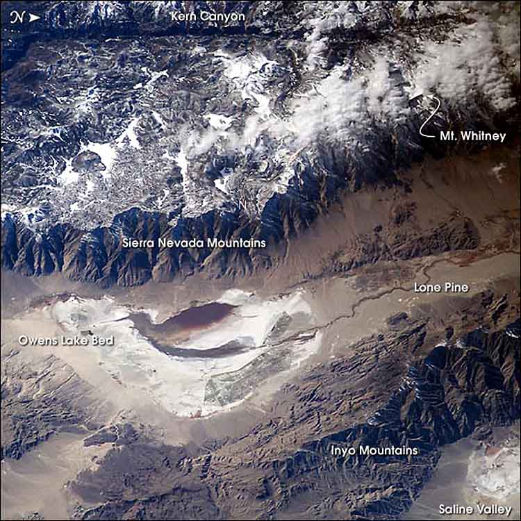
Figure 13.3: Photo taken from the ISS showing the Sierra Nevada Mountains running from left to right; the mountain range on the upward side of the image are snow capped while the mountain slopes and basin at the base of the range on the downward side of the image are tan and lack vegetation, indicating a rain shadow. The Inyo Mountains are near the bottom of the photo which lack snow due to the rain shadow.
Figure 13.4: An illustration of the Earth with three generalized circulation cells shown for each hemisphere; the Polar cell is located above 50 degrees north and south latitude, the Mid-latitude cell is located between 30 and 50 degrees north and south latitude, and the Hadley cell is located between 0 and 30 degrees north and south latitude. On the globe, arrows show the general wind directions in each cell: polar winds flow outward from each pole in the Polar cells, westerlies flow from west to east, toward the poles in the Mid-latitude cells, northeasterly trades flow from the northeast to southwest in the northern Hemisphere Hadley cell, and southeasterly trades flow from the southeast to northwest in the southern Hemisphere Hadley cell.
Figure 13.5: Map of the Great Basin Desert, located across most of Nevada, Western Utah, southeastern Idaho, and eastern California. The Humboldt River runs approximately east to west in the northern part of the desert and the Great Salt Lake is located near the eastern edge of the desert.
Figure 13.6: Map of South America with the Atacama Desert colored yellow and orange: the desert is located along the coast of west-central South America.
Figure 13.7: Circular map of the northern hemisphere centered on the North Pole. The map is color coded according to geopotential height, with cold, descending air in purple over the Arctic.
Figure 13.8: Animation illustrating a ball thrown on a rotating disc viewed from two perspectives: from the inertial frame of reference and from a stationary viewer on the disc. Viewed from the inertial frame of reference, the ball moves in a straight line from the center of the disc to the bottom of the image as the disc rotates counterclockwise. Viewed from the perspective of a stationary viewer on the disc, the ball appears to follow a curved path from the center outward toward the left of the viewer.
Figure 13.9: Schematic diagram showing forces acting on a mass moving East or West on the rotating Earth. As the Earth rotates, centripetal force pushes the mass outward while gravity force pulls the mass toward the center of Earth; combined, the Coriolis effect is between these two forces.
Figure 13.10: Illustration of the Earth with circular arrows pointing clockwise in the Northern Hemisphere and counterclockwise in the Southern Hemisphere, which equates to Coriolis deflection to the right in the Northern Hemisphere and to the left in the Southern Hemisphere.
Figure 13.11: World map of ocean currents; in the northern hemisphere, large-scale gyres flow in a clockwise pattern in each ocean basin; in the southern hemisphere, large-scale gyres flow in a counterclockwise pattern in each ocean basin. Cool currents are generally found along the west coasts of continents and are blue in color; warm currents are generally found along the east coasts of continents and are red in color; the rest of the currents are black.
Figure 13.12: Photo through a sandstone arch of a desert landscape with steep sandstone cliffs, distant spires, and a flat basin.
Figure 13.13: The rock is dark brown with tan petroglyphs carved into it.
Figure 13.14: A few trucks on dry, flat land. From ground to sky is a dark brown dust cloud that you cannot see through.
Figure 13.15: 2D diagram showing how sand grains can travel by wind blowing on a sandy ground surface: the largest grains move along the ground surface and are labeled creep, slightly smaller particles bounce along the surface and are labeled saltation, and tiny particles that move through the air are labeled suspension.
Figure 13.16: Close-up photo of unconsolidated amber-colored glassy grains with rounded edges; a scale bar at the lower right says 1.0 mm.
Figure 13.17: A large gray rock has slid over the light tan playa surface leaving a track in the playa.
Figure 13.18: Top photo shows sand-covered ground that has a sandstone rock resting on top of a base that has been worn away by sandblasting. Bottom photo shows man standing in bowl-shaped sandy depression.
Figure 13.19: Column of sand with larger sand boulder capping the column; the boulder has multiple flattened and faceted surfaces.
Figure 13.20: Black and white aerial image with white elevation contour lines overlain on the image. The contour lines show a semi-circular fan-shaped deposit where a stream emerges from a canyon in Death Valley.
Figure 13.21: Photo of mountains where alluvial fans have coalesced into a single apron of sediment along the mountain front.
Figure 13.22: Single dome-shaped mountain rising from a flat desert landscape.
Figure 13.23: Satellite image of a flat tan desert playa surrounded by mountains on either side.
Figure 13.24: Top photo shows a dry sandy stream bed surrounded by a desert landscape with scrubby vegetation, while the bottom photo shows a tan muddy water flooding in the desert.
Figure 13.25: Left photo shows a tan sandy desert landscape with a yellow sign that states warning flash flood area. Right photo shows a person standing in a very narrow tan sandy canyon.
Figure 13.26: Vast tan, sandy desert landscape. A single person and a white vehicle can be seen in the distance.
Figure 13.27: Cross sectional diagram showing wind blowing toward the right and sand moving as a result. There are three flat-lying sedimentary beds with smaller cross beds angled from upper left to lower right across the beds. Erosion happens on the gently-sloping left-hand side of the bed surface while deposition happens on the steeper right-hand side of the bed surface.
Figure 13.28: Tan sandstone with many thinly-bedded layers at various angles visible along the cliff face.
Figure 13.29: Satellite image of a field of barchan dunes, each showing characteristic crescent shapes with the wings pointing in the direction of prevailing winds.
Figure 13.30: Satellite image of long, linear parallel dune ridges in a tan sandy landscape.
Figure 13.31: Block diagram of a beach with wind blowing toward the left. Parabolic dunes form in the sand that have a crescent shape, with the horns anchored in vegetation and pointing toward the right. A bowl-shaped blowout forms in the sand where there is no vegetation.
Figure 13.32: Tan sand dune with a central peak and multiple ridges branching outward in various directions.
Figure 13.33: Map of the Great Basin Desert, located across most of Nevada, Western Utah, southeastern Idaho, eastern California, and south-central Oregon. Multiple streams begin and end within the basin.
Figure 13.34: Desert landscape covered in low scrubby vegetation. A town can be seen in the distance.
Figure 13.35: World map color coded according to desert vulnerability: low vulnerability is light green, moderate is yellow, high is orange, and very high is red. Regions with high and moderate vulnerability include western and southwestern U.S., eastern and south-central South America, sub- Saharan Africa and southern Africa, the Middle East, and the coastal regions of Australia. Other regions either have low to moderate vulnerability or are classified as other regions: dry, cold, humid/not vulnerable, or ice/glacier.
Figure 13.36: A long sheet of ice filling an alpine valley with parallel lines of sediment running lengthwise along the ice. In the background is a thick deposit of ice higher up in a mountain cirque.
Figure 13.37: Aerial photo of a mountainous terrain; the mountain slopes are dark brown, capped with a large expanse of white snow and ice; a deep blue lake can be seen in a valley on the right side of the photo.
Figure 13.38: Left image is an aerial photo of a broad expanse of white snow and ice. There are numerous waterways off the right side of the ice sheet. Right image is a map of Greenland showing the thickness of the ice sheet that covers nearly the entire country. The ice is thickest near the center of Greenland with a maximum thickness of 3,205 meters and gets thinner outward toward the coasts.
Figure 13.39: Antarctic ice sheet is very wide (roughly 6,000km). Greenland ice sheet is narrower (roughly 1,000 km). Both ice sheets have roughly the same height. Crust of each ice sheet remains at or below sea level.
Figure 13.40: Two photos: the left photo shows the side profile of a rocky mountain that is covered with an ice cap. The right photo is an aerial view of a white ice cap covering a large area of land.
Figure 13.41: Map centered over the North Pole, showing the maximum extent of the Laurentide ice sheet. The ice sheet covers Greenland, Canada, the northern United States, northern Europe, and northern Asia.
Figure 13.42: Two photos: the left photo shows deep cracks in a sheet of glacial ice and the right photo shows a person stepping over a deep crack in a sheet of glacial ice.
Figure 13.43: Cross sectional diagram of a glacier on a slope with elevation on the vertical axis. The glacier flows downhill at different rates with red numbers showing the stress on the ice in kilopascals and arrows showing the relative extent of deformation. In general, the stress increases deeper below the glacier surface and deforms most along the base of the glacier.
Figure 13.44: A cross sectional diagram of an alpine glacier on a slope with internal flow lines shown as blue arrows that point downhill parallel to the slope. The zone of accumulation and zone of melting are separated by a vertical equilibrium line, with the zone of accumulation being upslope and the zone of ablation downslope.
Figure 13.45: Water-filled valley with steep side walls.
Figure 13.46: Two photos: the left photo shows a big, smooth rock with parallel linear grooves and the right photo shows smoothed, polished rock with parallel linear grooves abraded.
Figure 13.47: A U-shaped valley with steep ridges on the sides and a wide curved valley at the base.
Figure 13.48: Animated GIF of the formation of a glacial valley: the valley begins as a V- shaped valley with a river running through it. As ice forms on the mountains and fills the valley, the glacier then carves away at the base of the valley, changing it into a U-shaped valley. At the end of the animation, the ice melts away and leaves behind a U-shaped glacial valley with a few rivers and a lake at the base.
Figure 13.49: Three photos: the left photo shows a steep rocky mountain that has an amphitheatre-like valley carved out of the top of the mountain, with a lake at the base. The middle photo shows a steep and pointy rocky mountain top. The right photo shows a steep rocky mountain with a U-shaped valley halfway up the slope; a large waterfall flows out of the mid-height valley onto the valley below.
Figure 13.50: A large boulder, dark in color, with smaller lighter colored clasts of a range of sizes inside of it.
Figure 13.51: Two photos: the left photo shows a long sheet of ice at the base of mountains with parallel lines of sediment running lengthwise along the ice, resembling an ice road. The right photo shows two long sheets of ice at the base of mountains that meet in a Y-shape; both sheets have parallel lines of sediment running lengthwise along the ice, resembling an ice road.
Figure 13.52: Aerial photograph of a small town surrounded by green landscape; numerous elongated asymmetrical teardrop-shaped hills are seen surrounding the town, which is also located on a small ridge.
Figure 13.53: An elongated green valley with a light milky blue lake at the valley base. There are steep brown mountain cliffs in the background that have white snow covering part of them.
Figure 13.54: Series of elongate lakes between moraines within an alpine glacial valley.
Figure 13.55: Satellite view of a series of long, finger-shaped lakes next to each other over a large area.
Figure 13.56: Map showing a large lake covering southeastern Manitoba, northwestern Ontario, northern Minnesota, eastern North Dakota, and Saskatchewan.
Figure 13.57: Aerial photo of a barren and pockmarked terrain.
Figure 13.58: Map of the western United States showing present day lakes, Pleistocene lakes, and the Pleistocene ice sheet; Lake Bonneville is a Pleistocene lake in northwestern Utah and arrows show that it floods toward the northwest, along the Snake River, until it reaches the Scablands of eastern Washington; the modern Great Salt Lake is in the northern part of Lake Bonneville and is much smaller than Lake Bonneville. The ice sheet is located in Canada and the northern United States; it also floods toward the Scablands. Other smaller Pleistocene lakes are scattered across the western U.S.
Figure 13.59: Aerial view of the five great lakes (Superior, Huron, Michigan, Erie, Ontario) that occupy basins left by the ice sheet in the Ice Age.
Figure 13.60: A graph of atmospheric CO2 levels over time. The vertical axis shows Benthic O-18 in per mil, decreasing upward; the horizontal axis shows the time from 65 to 0 million years ago. During the Cenozoic Era, carbon dioxide levels steadily decreased from a maximum in the Paleocene, causing the climate to gradually cool. By the Pliocene, ice sheets began to form. There are short-term cycles of warming and cooling within the larger glaciation event.
Figure 13.61: World map, color coded by vertical crustal motions in mm per year. The highest rebound rate is 18.0 mm per year and high motions are indicated the blue-to-purple zones (top end of the scale). The lowest rebound rate is negative 6.0 mm per year, indicating isostatic lowering; these are orange- to-red zones (bottom end of the scale). Most glacial isostatic rebound is occurring where continental ice sheets rapidly melted about 19,000 years ago, such as in Canada, Scandinavia, and western Antarctica, and most isostatic lowering is occurring in the northern Atlantic Ocean and Arctic Ocean, with small spots of lowering off the coast of western Antarctica.
Desert that forms near 30° latitude due to atmospheric circulation.
Deserts that form as air loses moisture traveling over mountains.
Deserts formed by descending air at the poles.
Angle between a light ray that hits the ground and a line perpendicular at the point of contact with the ground. If the sun is directly above a point and light rays are hitting the ground directly, then the angle of incidence is 0.
A part of the global circulation system that rises at the equator and sinks at 30°.
Wind patterns that move from east to west near the equator due to global circulation patterns.
Winds that move from west to east between 30° and 60° latitude due to global circulation patterns.
Desert area stretching east from California to Utah and north to Idaho/Oregon; formed due to both latitude and rain shadow.
Driest nonpolar desert on Earth, located in west-central South America.
Part of the global circulation pattern in which air sinks at the poles (90° latitude) and rises at 60° latitude.
Dark mineralization that forms on rocks in desert environments.
A dust storm that occurs in desert areas.
Silt and sand that is lifted from the bed and transported short distances.
Rocks that move along thin ice sheets with high winds.
Erosional rock face caused by sand abrasion.
Rock with abraded surfaces formed in deserts.
A depression in dune sediment formed because of a lack of anchoring vegetation.
Loose sediment deposited from running water.
A group of several alluvial fans that have come together and formed a single surface.
Isolated piece of bedrock that protrudes from an alluvial surface.
Planar flow of water over land surfaces.
Dry riverbed in an arid region.
A vast stretch of sand dunes.
Slope angle where shear forces and normal forces are equal.
Crescent-shaped dune formed by consistent wind and limited sediment.
Dunes that are much longer than they are wide, forming from wind blowing in two opposite directions.
Dunes that form semicircular shapes due to anchoring vegetation.
Dunes that form from wind of many different directions.
The process that turns nondesert land into desert.
A body of ice that moves downhill under its own mass.
Snow that has been compressed and is starting to turn into ice.
An alpine glacier that fills a mountain valley.
A glacier that forms on a mountain.
Thick glaciers that cover continents, particularly during ice ages.
A body of ice covering large stretches of land over a continent (mainly found in Antarctica).
A crack that forms with glacial movement in the upper, brittle part of the glacier.
The net gain or loss of ice within a glacier.
Part of a glacier that has shown a net gain of material over the course of a year.
The line between the zone of accumulation and the zone of ablation.
A process where ice from the ends of glaciers falls into the ocean.
Smooth surface carved in hard rocks by glacial action.
Grooves scratched in rock by glacial action.
A ridge that is carved between two glacial valleys.
Glacially-carved, bowl-shaped valley.
Steep spire carved by several glaciers.
An eroded arête that forms a triangular shape.
General term for very poorly sorted sediment that is of glacial origin.
A rock made definitively of glacial till.
Accumulation of sediment at the margins of glaciers, including the base, sides, and end.
Moraine that forms at the end of a glacier.
A terminal moraine that forms as a glacier melts.
Moraines that form at the sides of glaciers.
Formed by two or more glaciers merging, with lateral moraines combining to form a moraine within the glacier.
An accumulation of sediment that forms beneath a glacier.
Accumulation of fine-grained sediment formed downhill of the terminal moraine.
Large sediment (e.g., boulder) carried and then dropped by a glacier.
Depression formed by ice resting in sediment, then preserved after the ice melts and the sediment lithifies.
Ridge of sediment that forms under a glacier by meltwater that has formed a river.
Ridge of sediment that forms under a glacier with steep uphill and gentle downhill sides in respect to the glacier.
A series of lakes between moraines within an alpine glacier basin, typically a cirque.
Lake that fills a glacial valley.
Lake that forms next to a glacier because of crustal loading.
Lakes that form via increased precipitation from glacial climate shifts.
A period of cooler temperatures on Earth in which ice sheets can grow on continents.
A series of changes in the Earth's orbit/position in relation to the Sun, which can cause climates to fluctuate over periodicities.
Wobbles in the Earth's axis.
The angle of the Earth's axis with respect to the plane of rotation.
The measure of the circular or elliptical nature of the Earth's orbit.
Referring to overall global sea level change, either due to climate or seafloor spreading rate.
An upward movement of the lithosphere when weight is removed, such as water or ice.
An exposed coastline where relative sea level is falling.
