15 Global Climate Change

This chapter describes the Earth systems involved in climate change, the geologic evidence of past climate changes, and the human role in today’s climate change. In science, a system is a group of interacting objects and processes. Earth system science is the study of these systems: geosphere (rocks), atmosphere (gases), hydrosphere (water), cryosphere (ice), and biosphere (living things). Earth science studies these systems and how they interact and change in response to natural cycles and anthropogenic (human-driven) forces. Changes in one Earth system affect other systems.

It is critically important for us to be aware of the geologic context of climate change processes and how these Earth systems interact, first, for us to understand how and why human activities cause present-day climate change and, second, to distinguish between natural processes and human processes in the geologic past’s climate record.

A significant part of this chapter introduces and discusses various processes from these Earth systems, how they influence each other, and how they impact global climate. For example, Earth’s temperature and climate largely change based on atmospheric gas composition, ocean circulation, and the land-surface characteristics of rocks, glaciers, and plants.

As previously mentioned in the Meteorology chapter, understanding climate change requires the ability to distinguish between climate and weather. Weather is the short-term temperature and precipitation patterns that occur in days and weeks. Climate is the variable range of temperature and precipitation patterns averaged over the long-term for a particular region (see Section 13.1). Thus, a single cold winter does not mean that the entire globe is cooling; indeed, the United States’ cold winters of 2013 and 2014 occurred while the rest of the Earth was experiencing record warm-winter temperatures. To avoid these generalizations, many scientists use a 30-year average as a good baseline. Therefore, climate change refers to slow temperature and precipitation changes and trends over the long term for a particular area or the Earth as a whole.

15.1 Earth’s Temperature

Without an atmosphere, Earth would have huge temperature fluctuations between day and night, as the Moon does. Daytime temperatures would be hundreds of degrees Celsius above normal, and nighttime temperatures would be hundreds of degrees below normal. Because the Moon doesn’t have much of an atmosphere, its daytime temperatures are around 106°C (223°F) and nighttime temperatures are around -183°C (-298°F). That is an astonishing 289°C (521°F) degree range between the Moon’s light side and dark side. This section describes how Earth’s atmosphere is involved in regulating the Earth’s temperature.

15.1.1 Composition of Atmosphere

The atmosphere’s composition is a key component in regulating the planet’s temperature. The atmosphere is 78% nitrogen (N₂), 21% oxygen (O₂), 1% argon (Ar), and less than 1% trace components, which are all other gases. Trace components include carbon dioxide (CO₂), water vapor (H₂O), neon, helium, and methane. Water vapor is highly variable, mostly based on region, and composes about 1% of the atmosphere. Trace component gases include several important greenhouse gases, which are the gases responsible for warming and cooling the plant. On a geologic scale, volcanoes and the weathering process, which bury CO₂ in sediments, are the atmosphere’s CO₂ sources. Biological processes both add and subtract CO₂ from the atmosphere.

Greenhouse gases trap heat in the atmosphere and warm the planet by absorbing some of the longer-wave outgoing infrared radiation that is emitted from Earth, thus keeping heat from being lost to space. More greenhouse gases in the atmosphere absorb more longwave heat and make the planet warmer. Greenhouse gases have little effect on shorter-wave incoming solar radiation.

The most common greenhouse gases are water vapor (H₂O), carbon dioxide (CO₂), methane (CH₄), and nitrous oxide (N₂O). Water vapor is the most abundant greenhouse gas, but its atmospheric abundance does not change much over time. Carbon dioxide is much less abundant than water vapor, but carbon dioxide is being added to the atmosphere by human activities such as burning fossil fuels, land-use changes, and deforestation. Further, natural processes such as volcanic eruptions add carbon dioxide, but this occurs at an insignificant rate compared to human-caused contributions.

There are two important reasons why carbon dioxide is the most important greenhouse gas. First, carbon dioxide stays in the atmosphere and does not go away for hundreds of years. Second, most of the additional carbon dioxide is “fossil” in origin, which means that it is released by burning fossil fuels. For example, coal and petroleum are fossil fuels. Coal and oil are made from long-dead plant material, which was originally created by photosynthesis millions of years ago and stored in the ground. Photosynthesis combines sunlight and carbon dioxide to create the substances of plants. This transformation occurs over millions of years as a slow process, accumulating fossil carbon in rocks and sediments. So, when we burn coal and oil, we instantaneously release the stored solar energy and fossil carbon dioxide that took millions of years to accumulate in the first place. The rate of release is critical to comprehend current climate change.

15.1.2 Carbon Cycle

Understanding global climate change requires an understanding of the carbon cycle and how Earth’s own carbon-balancing system is being rapidly thrown off balance by human-driven activities. Earth has two important carbon cycles: the biological and the geological. In the biological cycle, living organisms—mostly plants—consume carbon dioxide from the atmosphere to make their tissues and substances through photosynthesis. Then, after the organisms die and then decay over years or decades, that carbon is released back into the atmosphere. The following is the general equation for photosynthesis.

CO₂ + H₂O + sunlight → sugars + O₂

In the geological carbon cycle, a portion of the biological-cycle carbon becomes part of the geological carbon cycle: plant materials into coal and petroleum, tiny fragments and molecules into organic-rich shale, and the carbonate-bearing calcareous shells and other parts of marine organisms into limestone. Such materials become buried and become part of the slow geologic formation of coal and other sedimentary materials. This cycle actually involves most of Earth’s carbon and operates very slowly.

The following are geological carbon-cycle storage reservoirs:

• Organic matter from plants is stored in peat, coal, and permafrost for thousands to millions of years.
• Silicate-mineral weathering converts atmospheric carbon dioxide to dissolved bicarbonate, which is stored in the oceans for thousands to tens of thousands of years.
• Marine organisms convert dissolved bicarbonate to forms of calcite, which is stored in carbonate rocks for tens to hundreds of millions of years.
• Carbon compounds are directly stored in sediments for tens to hundreds of millions of years; some end up in petroleum deposits.
• Carbon-bearing sediments are transferred by subduction to the mantle, where the carbon may be stored for tens of millions to billions of years.
• Carbon dioxide from within the Earth is released back to the atmosphere during volcanic eruptions, where it is stored for years to decades.

During much of Earth’s history, the geological carbon cycle has been balanced by volcanoes releasing carbon at approximately the same rate that carbon is stored by the other processes. Under these conditions, Earth’s climate has remained relatively stable. However, in Earth’s history, there have been times when that balance has been upset. This can happen during prolonged stretches of above-average volcanic activity. One example is the Siberian Traps eruption around 250 million years ago, which contributed to strong climate warming over a few million years.

A carbon imbalance is also associated with significant mountain-building events. For example, the Himalayan Range has been forming for about 40 million years, and over that time—and still today—the rate of weathering on Earth has been enhanced because the huge mountains and extensive range present a greater surface area on which weathering takes place. The weathering of these rocks—most importantly the hydrolysis of feldspar—has resulted in consumption of atmospheric carbon dioxide and transfer of the carbon to the oceans and to ocean-floor carbonate-rich sediments. The steady drop in carbon dioxide levels over the past 40 million years, which contributed to the Pliocene-Pleistocene glaciations, is partly attributable to the formation of the Himalayan Range.

Another, nongeological form of carbon-cycle imbalance is happening today on a very rapid timescale. In just a few decades, humans have extracted volumes of fossil fuels, such as coal, oil, and gas stored in rocks over the past several hundred million years, and converted these fuels to energy and carbon dioxide. By doing so, we are changing the climate faster than has ever happened in the past. Remember, carbon dioxide stays in the atmosphere and does not go away for hundreds of years. The more greenhouse gases in the atmosphere, the more heat is trapped and the warmer the planet becomes.

15.1.3 Greenhouse Effect

The greenhouse effect is the reason our global temperature is rising, but it’s important to understand what this effect is and how it occurs. The greenhouse effect occurs because greenhouse gases are present in the atmosphere. The greenhouse effect is named after a similar process that warms a greenhouse or a car on a hot summer day. Sunlight passes through the glass of the greenhouse or car, reaches the interior, and changes into heat. The heat radiates upward and gets trapped by the glass windows. The greenhouse effect for the Earth can be explained in three steps.

Step 1: Solar radiation from the Sun is composed of mostly ultraviolet (UV) light, visible light, and infrared (IR) radiation. Components of solar radiation include parts with a shorter wavelength than visible light, like ultraviolet light, and parts of the spectrum with longer wavelengths, like IR and others. Some of the radiation gets absorbed, scattered, or reflected by the atmospheric gases, but about half of the solar radiation eventually reaches the Earth’s surface.

Step 2: The visible, UV, and IR radiation that reaches the surface converts to heat energy. Most students have experienced sunlight warming a surface such as pavement, a patio, or deck. When this occurs, the warmer surface then emits thermal radiation, which is a type of IR radiation. Then there is a conversion from visible, UV, and IR to just thermal IR. This thermal IR is what we experience as heat. If you have ever felt heat radiating from a fire or a hot stovetop, then you have experienced thermal IR.

Step 3: Thermal IR radiates from the Earth’s surface back into the atmosphere. But since it is thermal IR instead of UV, visible, or regular IR, this thermal IR gets trapped by greenhouse gases. In other words, the Sun’s energy leaves the Earth at a different wavelength than it enters, so the Sun’s energy is not absorbed in the lower atmosphere when energy is coming in, rather occurring when the energy is going out. The gases that are mostly responsible for this energy blocking on Earth include carbon dioxide, water vapor, methane, and nitrous oxide. The presence of more greenhouse gases in the atmosphere results in more thermal IR being trapped. Explore this external link to an interactive animation on the greenhouse effect from the National Academy of Sciences.

15.1.4 Earth’s Energy Budget

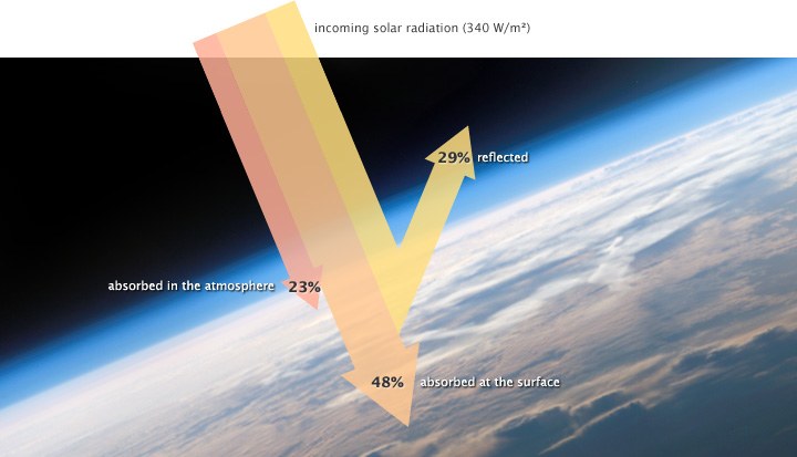
The solar radiation that reaches Earth is relatively uniform over time. Earth is warmed, and energy or heat radiates from the Earth’s surface and lower atmosphere back to space. This flow of incoming and outgoing energy is Earth’s energy budget. For Earth’s temperature to be stable over long stretches of time, incoming energy and outgoing energy have to be equal on average so that the energy budget at the top of the atmosphere balances. About 29% of the incoming solar energy arriving at the top of the atmosphere is reflected back to space by clouds, atmospheric particles, or reflective ground surfaces like sea ice and snow. About 23% of incoming solar energy is absorbed in the atmosphere by water vapor, dust, and ozone. The remaining 48% passes through the atmosphere and is absorbed at the surface. Thus, about 71% of the total incoming solar energy is absorbed by the Earth system.

When this energy reaches Earth, the atoms and molecules that make up the atmosphere and surface absorb the energy, and Earth’s temperature increases. If this material only absorbed energy, then the temperature of the Earth would continue to increase and eventually overheat. For example, if you continuously run a faucet in a stopped-up sink, the water level rises and eventually overflows. However, temperature does not infinitely rise because the Earth is not just absorbing sunlight; it is also radiating thermal energy or heat back into the atmosphere. If thetemperature of the Earth rises, the planet emits an increasing amount of heat to space, and this is the primary mechanism that prevents Earth from continually heating.

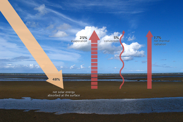
Some of the thermal infrared heat radiating from the surface is absorbed and trapped by greenhouse gases in the atmosphere, which act like a giant canopy over Earth. The more greenhouse gases in the atmosphere, the more outgoing heat Earth retains and the less thermal infrared heat dissipates to space.

Factors beyond greenhouse gases can affect the Earth’s energy budget. Increasing solar energy can increase the energy Earth receives. However, these increases are very small over time. In addition, land and water will absorb more sunlight when there is less ice and snow to reflect the sunlight back to the atmosphere. For example, the ice covering the Arctic Sea reflects sunlight back to the atmosphere; this reflected light is called albedo. Furthermore, aerosols (dust particles) produced from burning coal, diesel engines, and volcanic eruptions can reflect incoming solar radiation and actually cool the planet.

While the effect of anthropogenic aerosols on the climate’s system is weak, the effect of human-produced greenhouse gases is not weak. Thus, the net effect of human activity is warming due to more anthropogenic greenhouse gases associated with fossil fuel combustion.

An effect that changes the planet can trigger feedback mechanisms that amplify or suppress the original effect. A positive feedback mechanism occurs when the output or effect of a process enhances the original stimulus or cause. Thus, it increases the ongoing effect. For example, the loss of sea ice at the North Pole makes that area less reflective, reducing albedo. This allows the surface air and ocean to absorb more energy in an area that was once covered by sea ice. Another example is melting permafrost. Permafrost is permanently frozen soil located in the high latitudes, mostly in the Northern Hemisphere. As the climate warms, more permafrost thaws, and the thick deposits of organic matter are exposed to oxygen and begin to decay. This oxidation process releases carbon dioxide and methane, which in turn causes more warming, which melts more permafrost, and so on.

A negative feedback mechanism occurs when the output or effect reduces the original stimulus or cause. For example, in the short term, more carbon dioxide (CO₂) is expected to cause forest canopies to grow, which absorb more CO₂. Another example for the long term is that increased carbon dioxide in the atmosphere will cause more carbonic acid and chemical weathering, which results in the transportation of dissolved bicarbonate and other ions to the oceans, which are then stored in sediment.

Global warming is evidence that Earth’s energy budget is not balanced. Positive feedback on Earth’s temperature is now greater than negative feedback.

15.2 Evidence of Recent Climate Change

While climate has changed often in the past due to natural causes (see Section 14.5.1 and Section 15.3), the scientific consensus is that human activity is causing very rapid climate change. While this seems like a new idea, it was suggested more than 75 years ago. This section describes the evidence of what most scientists agree is anthropogenic or human-caused climate change. For more information, watch the video below on climate change by two professors at the North Carolina State University.

15.2.1 Global Temperature Rise

The land-ocean temperature index, 1880 to present, compared to a base reference time of 1951–1980, shows ocean temperatures steadily rising. The solid black line is the global annual mean, and the solid red line is the five-year Lowess smoothing. The blue uncertainty bars (95% confidence limit) account only for incomplete spatial sampling.

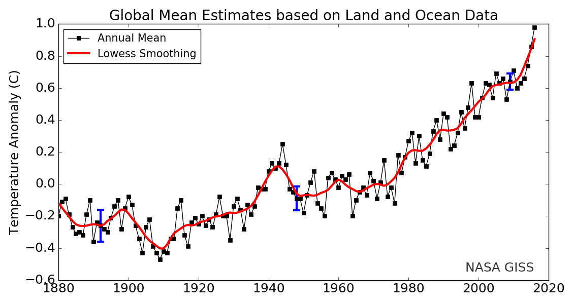
Since 1880, Earth’s surface-temperature average has trended upward, with most of that warming occurring since 1970 (see this NASA animation). Surface temperatures include both land and ocean because water absorbs much additional trapped heat. Changes in land-surface or ocean-surface temperatures compared to a reference period from 1951 to 1980, where the long-term average remained relatively constant, are called temperature anomalies. A temperature anomaly thus represents the difference between the measured temperature and the average value during the reference period. Climate scientists calculate long-term average temperatures over thirty years or more, which identified the reference period from 1951 to 1980. Another common range is a century, for example, 1900–2000. Therefore, an anomaly of 1.25°C (2.25°F) for 2015 means that the average temperature for 2015 was 1.25°C (2.25°F) greater than the 1900–2000 average. In 1950, the temperature anomaly was -0.28°C (-0.504°F), so this is -0.28°C (-0.504°F) lower than the 1900–2000 average. These temperatures are annual average measured surface temperatures.

This video of temperature anomalies shows worldwide temperature changes since 1880. The more blue, the cooler; the more yellow and red, the warmer.

In addition to average land-surface temperatures rising, the ocean has absorbed much heat. Because oceans cover about 70 percent of the Earth’s surface and have such a high specific heat value, they provide a large opportunity to absorb energy. The ocean has been absorbing about 80-to-90 percent of human activities’ additional heat. As a result, the top 700 meters (2,300 feet) of the global ocean has warmed about 0.83°C (1.5°F) since 1901 (watch this three-minute video by NASA JPL on the ocean’s heat capacity). The reason the ocean has warmed less than the atmosphere, while still taking on most of the heat, is due to water’s very high specific heat, which means that water can absorb a lot of heat energy with a small temperature increase. In contrast, the lower specific heat of the atmosphere means it has a higher temperature increase, as it absorbs less heat energy.

Some scientists suggest that anthropogenic greenhouse gases do not cause global warming because between 1998 and 2013, Earth’s surface temperatures did not increase much, despite greenhouse gas concentrations continuing to increase. However, since the oceans are absorbing most of the heat, decade-scale circulation changes in the ocean, similar to La Niña, push warmer water deeper under the surface. Once the ocean’s absorption and circulation is accounted for and this heat is added back into surface temperatures, then temperature increases become apparent. Also, the ocean’s heat storage is temporary, as reflected in the record-breaking warm years of 2014–2016. Indeed, with this temporary ocean-storage effect, 15 of the twenty-first century’s first 16 years were the hottest in recorded history.

15.2.2 Carbon Dioxide

Anthropogenic greenhouse gases, mostly carbon dioxide (CO₂), have increased since the Industrial Revolution, when humans dramatically increased burning fossil fuels. These levels are unprecedented in the last 800,000-year Earth history as recorded in geologic sources such as ice cores. Carbon dioxide has increased by 40 percent since 1750, and the rate of increase has been the fastest during the last decade. For example, since 1750, 2,040⁹ tonnes (2,040 gigatons) of CO₂ have been added to the atmosphere; about 40 percent has remained in the atmosphere, while the remaining 60 percent has been absorbed into the land by plants and soil or into the oceans. Indeed, during the lifetime of most young adults, the total atmospheric CO₂ has increased by 50 ppm, or 15 percent.

Charles Keeling, an oceanographer with Scripps Institution of Oceanography in San Diego, California, was the first person to regularly measure atmospheric CO₂. Using his methods, scientists at the Mauna Loa Observatory, Hawai’i, have constantly measured atmospheric CO₂ since 1957. NASA regularly publishes these measurements at https://keelingcurve.ucsd.edu. Go there now to see the very latest measurement. Keeling’s measured values have been posted in a curve of increasing values, called the Keeling curve. This curve varies up and down in a regular annual cycle, from summer when the plants in the Northern Hemisphere use CO₂ to winter when they are dormant. But the curve shows a steady CO₂ increase over the past several decades. This curve increases exponentially, not linearly, showing that the rate of CO₂ increase is itself increasing.

The following video shows how atmospheric CO₂ has varied recently and over the last 800,000 years, as determined by an increasing number of CO₂ monitoring stations (shown on the insert map). It is also instructive to watch the video’s Keeling portion of how CO₂ varies by latitude. This shows that most human CO₂ sources are in the Northern Hemisphere, which is home to most of the land and most of the developed nations.

15.2.3 Melting Glaciers and Shrinking Sea Ice

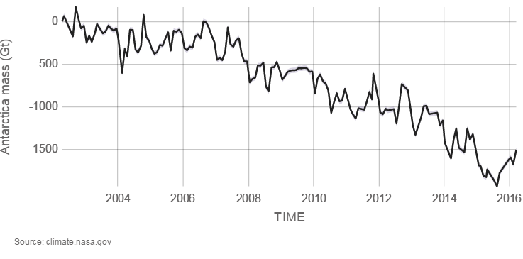
Glaciers are large ice accumulations that exist year-round on the land’s surface. In contrast, icebergs are masses of floating sea ice, although they may have had their origin in glaciers (see Glaciers chapter). Alpine glaciers, ice sheets, and sea ice are all melting. Explore melting glaciers at NASA’s interactive Global Ice Viewer. Satellites have recorded that Antarctica is melting at 1,189 tonnes (118 gigatons) per year, and Greenland is melting at 2,819 tonnes (281 gigatons) per year; 1 metric tonne is 1,000 kilograms (1 gigaton is over 2 trillion pounds). Almost all major alpine glaciers are shrinking, deflating, and retreating. The ice-mass loss rate is unprecedented—never observed before—since the 1940s, when quality records for glaciers began.

Before anthropogenic warming, glacial activity was variable with some retreating and some advancing. Now, spring snow cover is decreasing, and sea ice is shrinking. Most sea ice is at the North Pole, which is only occupied by the Arctic Ocean and sea ice. The NOAA animation shows how perennial sea ice has declined from 1987 to 2015. The oldest ice is white, and the youngest, seasonal ice is dark blue. The amount of old ice has declined from 20% in 1985 to 3% in 2015.

15.2.4 Rising Sea Level

Sea level is rising 3.4 millimeters (0.13 inches) per year and rose 0.19 meters (7.4 inches) from 1901 to 2010. This is largely thought to be from both glaciers melting and thermal expansion of seawater. Thermal expansion means that, as objects such as solids, liquids, and gases heat up, they expand in volume.

Below is a classic video demonstration (30 second) on thermal expansion with brass ball and ring (North Carolina School of Science and Mathematics).

15.2.5 Ocean Acidification

Since 1750, about 40 percent of new anthropogenic carbon dioxide has remained in the atmosphere. The remaining 60 percent gets absorbed by the ocean and vegetation. The ocean has absorbed about 30 percent of that carbon dioxide. When carbon dioxide gets absorbed in the ocean, it creates carbonic acid. This makes the ocean more acidic, which then has an impact on marine organisms that secrete calcium carbonate shells. Recall that hydrochloric acid reacts by effervescing with limestone rock made of calcite, which is calcium carbonate. A more acidic ocean is associated with climate change and is linked to thinning the carbonate shells of some sea snails (pteropods) and small protozoan zooplanktons (foraminifera) and to ocean coral reefs’ declining growth rates. Small animals like protozoan zooplankton are an important component at the base of the marine ecosystem. Combined with warmer temperature and lower oxygen levels, acidification is expected to have severe impacts on marine ecosystems and human-harvested fisheries, possibly affecting our ocean-derived food sources.

15.2.6 Extreme Weather Events

Extreme weather events such as hurricanes, precipitation, and heat waves are increasing and becoming more intense. Since the 1980s, hurricanes, which are generated from warm ocean water, have increased in frequency, intensity, and duration and are likely connected to a warmer climate. Since 1910, average precipitation has increased by 10 percent in the contiguous United States, and much of this increase is associated with heavy precipitation events. However, the distribution is not even, and more precipitation is projected for the Northern United States, while less precipitation is projected for the already dry Southwest. Also, heat waves have increased, and rising temperatures are already affecting crop yields in northern latitudes. Increased heat allows for greater moisture capacity in the atmosphere, increasing the potential for more extreme events.

15.3 Prehistoric Climate Change

Over Earth’s history, the climate has changed a lot. For example, during the Mesozoic Era, the Age of Dinosaurs, the climate was much warmer, and carbon dioxide was abundant in the atmosphere. However, throughout the Cenozoic Era, 65 million years ago to today, the climate has been gradually cooling. This section summarizes some of these major past climate changes.

15.3.1 Past Glaciations

Through geologic history, climate has changed slowly over millions of years. Before the most recent Pliocene-Quaternary glaciation, there were other major glaciations. The oldest, known as the Huronian, occurred toward the end of the Archean Eon-early Proterozoic Eon, about 2.5 billion years ago. The Great Oxygenation Event (see Chapter 8) occurred during that time and is most commonly associated with causing that glaciation. The increased oxygen is thought to have reacted with the potent greenhouse gas methane, causing cooling.

The end of the Proterozoic Eon, about 700 million years ago, had other glaciations. These ancient Precambrian glaciations are included in the snowball Earth hypothesis. Widespread global rock sequences from these ancient times contain evidence that glaciers existed even in low latitudes. Two examples are limestone rock—usually formed in tropical marine environments—and glacial deposits—usually formed in cold climates—from this time that have been found together in many regions around the world. One example is in Utah. Evidence of continental glaciation is seen in interbedded limestone and glacial deposits (diamictites) on Antelope Island in the Great Salt Lake.

The controversial snowball Earth hypothesis suggests that a runaway albedo effect—where ice and snow reflect solar radiation and increasingly spread from polar regions toward the equator—caused land and ocean surfaces to completely freeze and biological activity to collapse. Since carbon dioxide could not enter the then-frozen ocean, the ice covering Earth could only melt when volcanoes emitted high enough carbon dioxide into the atmosphere to cause greenhouse heating. Some studies estimate that, because of the frozen ocean surface, carbon dioxide 350 times higher than today’s concentration was required. Because biological activity did survive, the complete freezing and its extent in the snowball Earth hypothesis are controversial. A competing hypothesis is the slushball Earth hypothesis, in which some regions of the equatorial ocean remained open. Differing scientific conclusions about the stability of Earth’s magnetic poles, impacts on ancient rock evidence from subsequent metamorphism, and alternate interpretations of existing evidence keep the idea of snowball Earth controversial.

Glaciations also occurred in the Paleozoic Era, notably the Andean-Saharan glaciation in the late Ordovician, about 440–460 million years ago, which coincided with a major extinction event, and the Karoo ice age during the Pennsylvanian Period, 323–300 million years ago. This glaciation was one of the evidences cited by Wegener for his continental drift hypothesis as his proposed Pangea drifted into south polar latitudes. The Karoo glaciation was associated with an increase of oxygen and a subsequent drop in carbon dioxide, most likely produced by the evolution and rise of land plants.

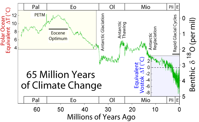
During the Cenozoic Era—the last 65 million years—climate started out warm and gradually cooled to its current state. This warm time is called the Paleocene-Eocene thermal maximum, and Antarctica and Greenland were ice-free during this time. Since the Eocene, tectonic events during the Cenozoic Era have caused the planet to persistently and significantly cool. For example, the Indian plate and Asian plate collided, creating the Himalaya Mountains, which increased the rate of weathering and erosion of silicate minerals, especially feldspar. Increased weathering consumes carbon dioxide from the atmosphere, which reduces the greenhouse effect, resulting in long-term cooling.

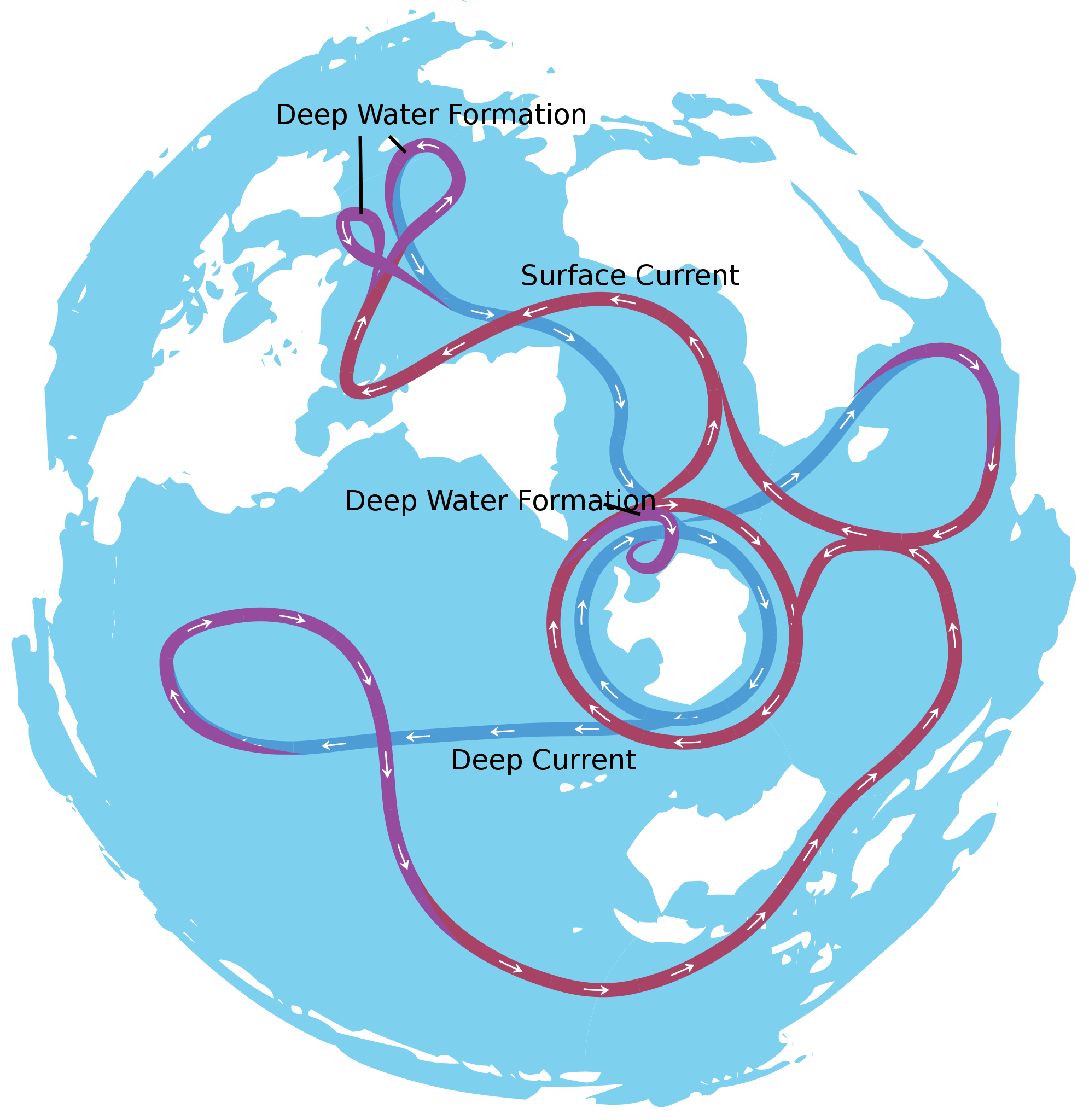
About 40 million years ago, the narrow gap between the South American plate and the Antarctica plate widened, which opened the Drake Passage. This opening allowed the water around Antarctica—the Antarctic Circumpolar Current—to flow unrestrictedly west to east, which effectively isolated the Southern Ocean from the warmer waters of the Pacific, Atlantic, and Indian Oceans. The region cooled significantly, and by 35 million years ago, during the Oligocene Epoch, glaciers had started to form on Antarctica.

Around 15 million years ago, subduction-related volcanoes between Central and South America created the Isthmus of Panama, which connected North and South America. This prevented water from flowing between the Pacific and Atlantic Oceans and reduced heat transfer from the tropics to the poles. This reduced heat transfer created a cooler Antarctica and larger Antarctic glaciers. As a result, the ice sheet expanded on land and water, increased Earth’s reflectivity, and enhanced the albedo effect, which created a positive feedback loop: more reflective glacial ice, more cooling, more ice, more cooling, and so on.

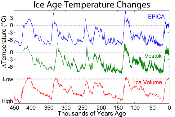
By five million years ago, during the Pliocene Epoch, ice sheets had started to grow in North America and Northern Europe. The most intense part of the current glaciation is the Pleistocene Epoch’s last million years. The Pleistocene’s temperature varies significantly through a range of almost 10°C (18°F) on timescales of 40,000 to 100,000 years, and ice sheets expand and contract correspondingly. These variations are attributed to subtle changes in Earth’s orbital parameters, called Milankovitch cycles.

As described in the Glaciers chapter, Milankovitch cycles are three orbital changes named after the Serbian astronomer Milutan Milankovitch. The three orbital changes are called precession, obliquity, and eccentricity. Precession is the wobbling of Earth’s axis with a period of about 21,000 years; obliquity is changes in the angle of Earth’s axis with a period of about 41,000 years; and eccentricity is variations in the Earth’s orbit around the Sun leading to changes in distance from the Sun with a period of 93,000 years. These orbital changes created a 41,000-year-long glacial-interglacial Milankovitch cycle from 2.5 to 1.0 million years ago, followed by another longer cycle of about 100,000 years from 1.0 million years ago to today (see Milankovitch cycles). Over the past million years, the glaciation cycles occurred approximately every 100,000 years, with many glacial advances occurring in the last two million years.

During an ice age, periods of warming climate are called interglacials; during interglacials, very brief periods of even warmer climate are called interstadials. These warming upticks are related to Earth’s climate variations, like Milankovitch cycles, which are changes to the Earth’s orbit that can fluctuate climate (see Glaciers chapter). In the last 500,000 years, there have been five or six interglacials, with the most recent belonging to our current time, the Holocene Epoch.

The two more recent climate swings, the Younger Dryas and the Holocene climatic optimum, demonstrate complex changes. These events are more recent yet have conflicting information. The Younger Dryas’ cooling is widely recognized in the Northern Hemisphere, though the event’s timing, about 12,000 years ago, does not appear to be equal everywhere. Also, it is difficult to find in the Southern Hemisphere. The Holocene climatic optimum is a warming around 6,000 years ago; it was not universally warmer, not as warm as current warming, and not warm at the same time everywhere.

15.3.2 Proxy Indicators of Past Climates

How do we know about past climates? Geologists use proxy indicators to understand past climate. A proxy indicator is a biological, chemical, or physical signature preserved in the rock, sediment, or ice record that acts like a fingerprint of something in the past. Thus, they are an indirect indicator of climate. An indirect indicator of ancient glaciations from the Proterozoic Eon and Paleozoic Era is the Mineral Fork Formation in Utah, which contains rock formations of glacial sediments such as diamictite (tillite); this dark rock has many fine-grained components plus some large out-sized clasts like a modern glacial till.

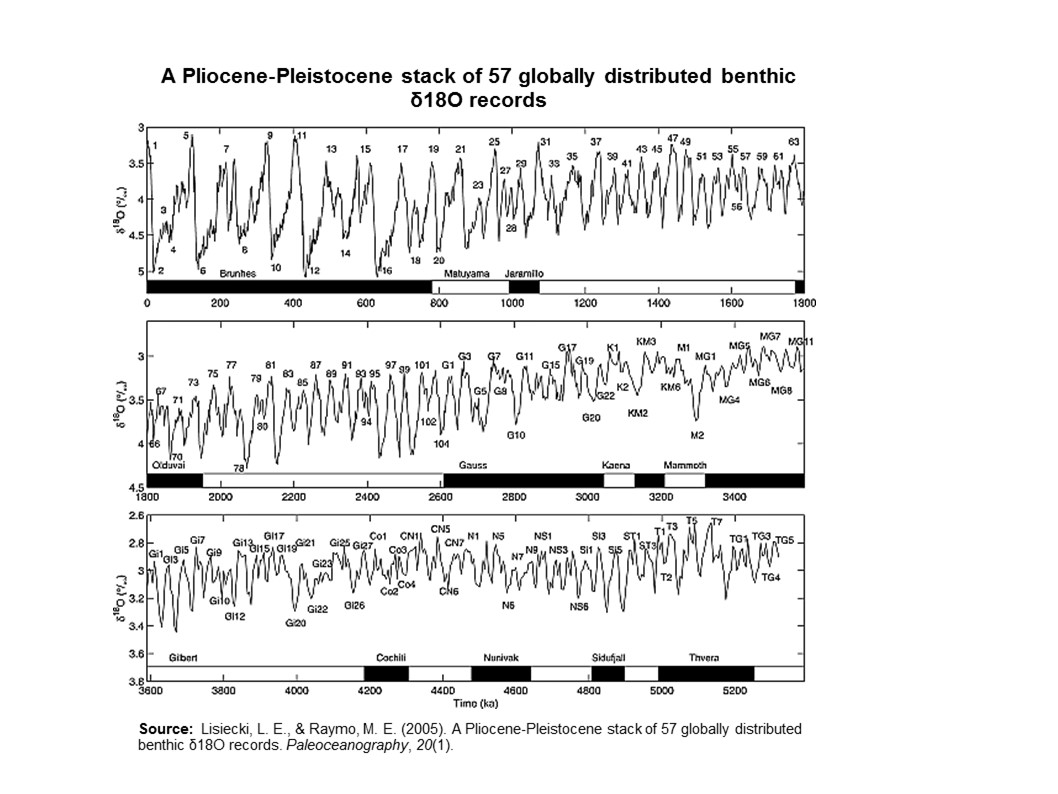
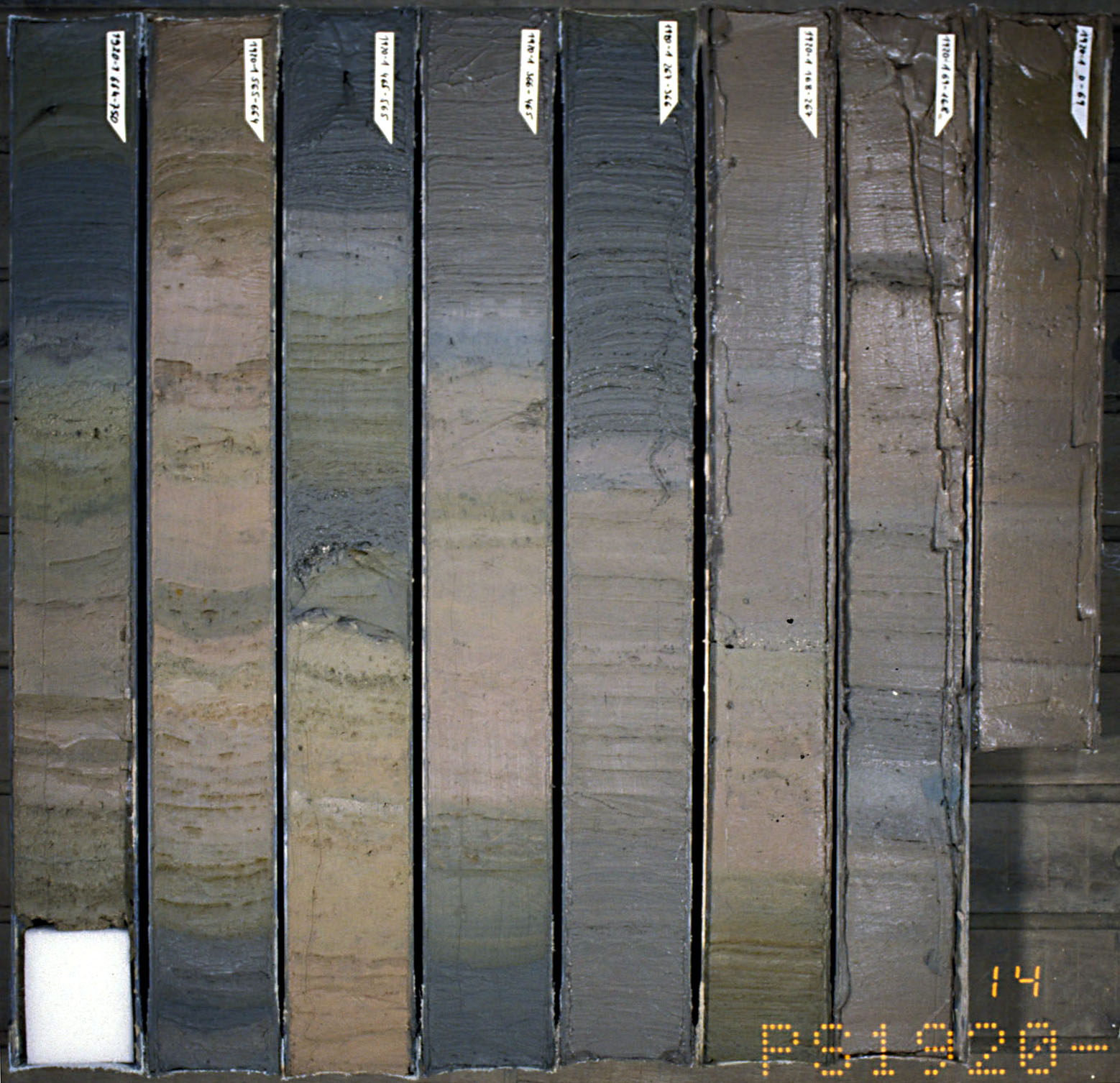
Deep-sea sediment is an indirect indicator of climate change during the Cenozoic Era. Researchers from the Ocean Drilling Program, an international research collaboration, collect deep-sea sediment cores that record continuous sediment accumulation. The sediment provides detailed chemical records of stable carbon and oxygen isotopes obtained from deep-sea benthic foraminifera shells that accumulated on the ocean floor over millions of years. The oxygen isotopes are a proxy indicator of deep-sea temperatures and continental ice volume.

Sediment Cores: Stable Oxygen Isotopes

How do oxygen isotopes indicate past climate? The two main stable oxygen isotopes are ¹⁶O and ¹⁸O. They both occur in water (H₂O) and in the calcium carbonate (CaCO₃) shells of foraminifera, acting as both of those substances’ oxygen component. The most abundant and lighter isotope is ¹⁶O. Since it is lighter, it evaporates more readily from the ocean’s surface as water vapor, which later turns to clouds and precipitation on the ocean and land. This evaporation is enhanced in warmer seawater and slightly increases the concentration of ¹⁸O in the surface seawater from which the plankton derives the carbonate for its shells. Thus, the ratio of ¹⁶O and ¹⁸O in the fossilized shells in seafloor sediment is a proxy indicator of the temperature and evaporation of seawater.

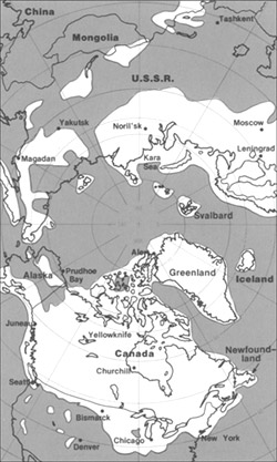
Keep in mind, it is harder to evaporate the heavier water and easier to condense it. As evaporated water vapor drifts toward the poles and tiny droplets form clouds and precipitation, droplets of water with ¹⁸O tend to form more readily than droplets of the lighter form and then precipitate out, leaving the drifting vapor depleted in ¹⁸O. During geologic times when the climate is cooler, more of this lighter precipitation that falls on land is locked in the form of glacial ice. Consider that the giant ice sheets were more than a mile thick and covered a large part of North America during the last ice age only 14,000 years ago. During glaciation, the glaciers effectively lock away more ¹⁶O, thus the ocean water and foraminifera shells become enriched in ¹⁸O. Therefore, the ratio of ¹⁸O to ¹⁶O (δ¹⁸O) in calcium carbonate shells of foraminifera is a proxy indicator of past climate. The sediment cores from the Ocean Drilling Program record a continuous accumulation of these fossils in the sediment and provide a record of glacials, interglacials and interstadials.

Sediment Cores: Boron-Isotopes and Acidity

Ocean acidity is affected by carbonic acid and is a proxy for past atmospheric CO₂ concentrations. To estimate the ocean’s pH (acidity) over the past 60 million years, researchers collected deep-sea sediment cores and examined the ancient planktonic foraminifera shells’ boron-isotope ratios. Boron has two isotopes: ¹¹B and ¹⁰B. In aqueous compounds of boron, the relative abundance of these two isotopes is sensitive to pH (acidity), hence CO₂ concentrations. In the early Cenozoic, around 60 million years ago, CO₂ concentrations were over 2,000 ppm and had higher pH, and they then started falling around 55 to 40 million years ago, with a noticeable drop in pH indicated by boron isotope ratios. The drop was possibly due to reduced CO₂ outgassing from ocean ridges, volcanoes and metamorphic belts, and due to increased carbon burial resulting from subduction and the Himalaya Mountains uplift. By the Miocene Epoch, about 24 million years ago, CO₂ levels were below 500 ppm, and by 800,000 years ago, CO₂ levels didn’t exceed 300 ppm.

Carbon Dioxide Concentrations in Ice Cores

For the recent Pleistocene Epoch’s climate, researchers get a more detailed and direct chemical record of the last 800,000 years by extracting and analyzing ice cores from the Antarctic and Greenland ice sheets. Snow accumulates on these ice sheets and creates yearly layers. Oxygen isotopes are collected from these annual layers, and the ratio of ¹⁸O to ¹⁶O (δ¹⁸O) is used to determine temperature as discussed above. In addition, the ice contains small bubbles of atmospheric gas as the snow turns to ice. Analysis of these bubbles reveals the composition of the atmosphere at these previous times.

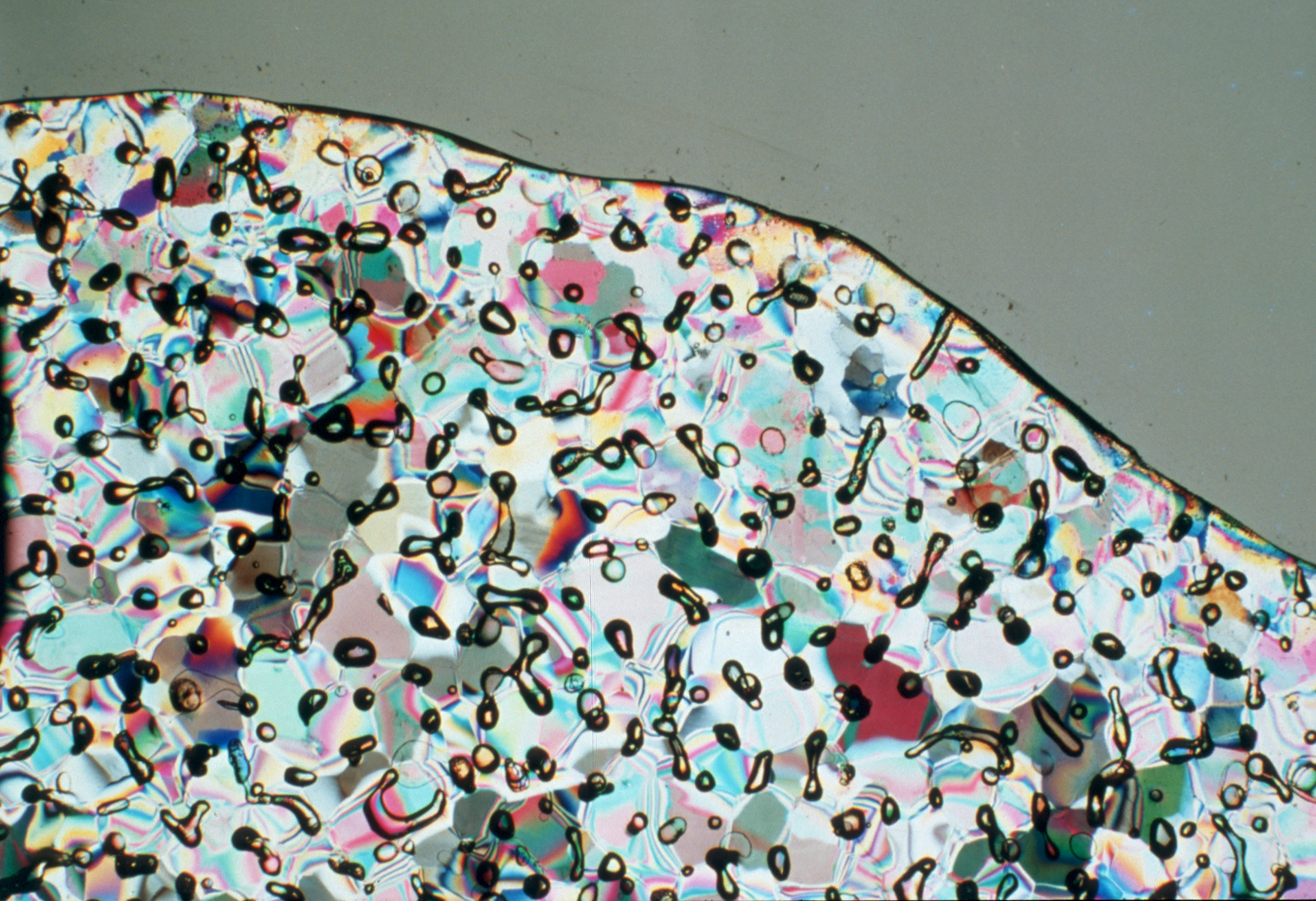
Small pieces of this ice are crushed, and the ancient air is extracted into a mass spectrometer that can detect the ancient atmosphere’s chemistry. Carbon dioxide levels are recreated from these measurements. Over the last 800,000 years, the maximum carbon dioxide concentration during warm times was about 300 parts per million (ppm), and the minimum was about 170 ppm during cold stretches. Currently, the Earth’s atmospheric carbon dioxide content is over 410 ppm.

Oceanic Microfossils

Microfossils like foraminifera, diatoms, and radiolarians can be used as proxies to interpret past climate record. Different species of microfossils are found in the sediment core’s different layers. Microfossil groups are called assemblages and their compositions differ depending on the climatic conditions when they lived. One assemblage consists of species that lived in cooler ocean water, such as in glacial times, while at a different level in the same sediment core, another assemblage consists of species that lived in warmer waters.

Tree Rings

Tree rings, which form every year as a tree grows, are another past climate indicator. Rings that are thicker indicate wetter years, and rings that are thinner and closer together indicate dryer years. Every year, a tree will grow one ring with a light section and a dark section. The rings vary in width. Since trees need much water to survive, narrower rings indicate colder and drier climates. Since some trees are several thousand years old, scientists can use their rings for regional paleoclimatic reconstructions—for example, to reconstruct past temperature, precipitation, vegetation, streamflow, sea-surface temperature, and other climate-dependent conditions. Paleoclimatic study means relating to a distinct past geologic climate. Dead trees, such as those found in Puebloan ruins, can be used to extend this proxy indicator by showing long-term droughts in the region, possibly explaining why villages were abandoned.

Pollen

Pollen is also a proxy climate indicator. Flowering plants produce pollen grains. Pollen grains are distinctive when viewed under a microscope. Sometimes, pollen is preserved in lake sediments that accumulate in layers every year. Lake-sediment cores can reveal ancient pollen. Fossil-pollen assemblages are pollen groups from multiple species, such as spruce, pine, and oak. Through time, via the sediment cores and radiometric age-dating techniques, the pollen assemblages change, revealing the plants that lived in the area at the time. Thus, pollen assemblages are a past climate indicator, since different plants will prefer different climates. For example, in the Pacific Northwest, east of the Cascades in a region close to grassland and forest borders, scientists tracked pollen over the last 125,000 years, covering the last two glaciations. Pollen assemblages with more pine tree pollen are found during glaciations, and pollen assemblages with less pine tree pollen are found during interglacial times.

Other Proxy Indicators

Paleoclimatologists study many other phenomena to understand past climates, such as human historical accounts, human instrument records from the recent past, lake sediments, cave deposits, and corals.

15.4 Anthropogenic Causes of Climate Change

As shown in the previous section, prehistoric climate changes occur slowly over many millions of years. The climate changes observed today are rapid and largely human caused. Evidence shows that climate is changing, but what is causing that change? Since the late 1800s, scientists have suspected that human-produced (i.e., anthropogenic) changes in atmospheric greenhouse gases would likely cause climate change because changes in these gases have been the cause every time in the geologic past. By the middle 1900s, scientists began conducting systematic measurements, which confirmed that human-produced carbon dioxide was accumulating in the atmosphere and other Earth systems, such as forests and oceans. By the end of the 1900s and into the early 2000s, scientists solidified the theory of anthropogenic climate change when evidence from thousands of ground-based studies and continuous land and ocean satellite measurements mounted, revealing the expected temperature increase. The theory of anthropogenic climate change states that humans are causing most of the current climate changes by burning fossil fuels such as coal, oil, and natural gas. Theories evolve and transform as new data and new techniques become available, and they represent a particular field’s state of thinking. This section summarizes the scientific consensus of anthropogenic climate change.

15.4.1 Scientific Consensus

The overwhelming majority of climate studies indicate that human activity is causing rapid changes to the climate, which will cause severe environmental damage. There is strong scientific consensus on the issue. Studies published in peer-reviewed scientific journals show that 97 percent of climate scientists agree that climate warming is caused from human activities. There is no alternative explanation for the observed link between human-produced greenhouse gas emissions and changing modern climate. Most leading scientific organizations endorse this position, including the US National Academy of Science, which was established in 1863 by an act of Congress under President Lincoln. Congress charged the National Academy of Science “with providing independent, objective advice to the nation on matters related to science and technology.” Therefore, the National Academy of Science is the leading authority when it comes to policy advice related to scientific issues.

One way we know that the increased greenhouse gas emissions are from human activities is through isotopic fingerprints. For example, fossil fuels, representing plants that lived millions of years ago, have a stable carbon-13 to carbon-12 (¹³C/¹²C) ratio that is different from today’s atmospheric stable-carbon ratio (radioactive ¹⁴C is unstable). Isotopic carbon signatures have been used to identify anthropogenic carbon in the atmosphere since the 1980s. Isotopic records from the Antarctic ice sheet show stable isotopic signatures from ~1000 CE to ~1800 CE and a steady isotopic signature gradually changing since 1800, followed by a more rapid change after 1950 as burning of fossil fuels dilutes the CO₂ in the atmosphere. These changes show the atmosphere as having a carbon isotopic signature increasingly more similar to that of fossil fuels.

15.4.2 Anthropogenic Sources of Greenhouse Gases

Anthropogenic emissions of greenhouse gases have increased since pre-industrial times due to global economic growth and population growth. Atmospheric concentrations of the leading greenhouse gas, carbon dioxide, are at unprecedented levels that haven’t been observed in at least the last 800,000 years. The pre-industrial level of carbon dioxide was at about 278 parts per million (ppm). In 2016, carbon dioxide was, for the first time, above 400 ppm for the entirety of the year. Measurements of atmospheric carbon at the Mauna Loa Carbon Dioxide Observatory show a continuous increase from 315 ppm since 1957 when the observatory was established to over 420 ppm in 2024. The daily reading today can be seen at Daily CO₂. Based on the ice core record over the past 800,000 years, carbon dioxide ranged from about 185 ppm during ice ages to 300 ppm during warm times. View the data-accurate NOAA animation below of carbon dioxide trends over the last 800,000 years.

What is the source of these anthropogenic greenhouse gas emissions? Fossil fuel combustion and industrial processes have contributed 78 percent of all emissions since 1970. The economic sectors responsible for most of this include electricity and heat production (25%); agriculture, forestry, and land use (24%); industry (21%); transportation, including automobiles (14%); other energy production (9.6%); and buildings (6.4%). More than half of greenhouse gas emissions have occurred in the last 40 years, and 40% of these emissions have stayed in the atmosphere. Unfortunately, despite scientific consensus, efforts to mitigate climate change require political action. Despite growing climate change concern, mitigation efforts, legislation, and international agreements have only reduced emissions in some places, while the less-developed world’s continual economic growth has increased global greenhouse gas emissions. In fact, the years 2000 to 2010 saw the largest increases since 1970.

15.4.3 Predicting Future Warming

Climate change can be a naturally occurring process and has created environments much warmer than today, such as the early Cretaceous Period. During this time, life thrived even in polar regions, such as the interior of Antarctica, which is uninhabitable today.

One misconception is that the threat of climate change has to do with the absolute warmth of the Earth. The concern for scientists has more to do with the rate of change of that temperature increase. Living organisms, including humans, can quickly adapt to substantial changes in climate if the changes take place slowly, over thousands of years. However, adapting to changes that are taking place on timescales of decades is far more challenging. The Earth is warming at such a rate that most species will struggle to adapt and evolve quickly enough to the coming warmer climates.

Prediction is difficult, especially about the future. This is also true for projections of future climate change, as they rely on assumptions about future radiative forcings such as anthropogenic emissions of greenhouse gases and aerosols, which are unknown. For this reason, they are called projections and not predictions.

Climate scientists believe that the best projections consider results from state-of-the-science climate models because they are syntheses of theoretical and empirical knowledge. However, climate models are imperfect. Uncertainties in future projections will therefore arise from assumptions about both future greenhouse gas emissions and climate model errors.

The Intergovernmental Panel on Climate Change (IPCC) is a United Nations body that evaluates climate change science and publishes comprehensive Assessment Reports, Special Reports, and Methodology Reports. The latest Assessment Report, AR6, includes contributions from three Working Groups finalized between August 2021 and April 2022 and from a Synthesis Report completed in March 2023. These reports provide insights into climate change, its impacts, risks, and mitigation options. They can be freely accessed online.

The most recent IPCC Assessment Report (AR6) uses future scenarios that specify anthropogenic radiative forcing and CO₂ concentrations. They are called Shared Socioeconomic Pathways (SSPs) and are followed by two numbers. The first indicates the socioeconomic narrative, and the second indicates the radiative forcing around the year 2100. For example, the scenario SSP5-8.5 uses the socioeconomic narrative 5 (Fossil Fueled Development) and reaches a radiative forcing of 8.5 W/m² in the year 2100, whereas scenario SSP1-1.9 uses the socioeconomic narrative 1 (Sustainability) and reaches a radiative forcing of 1.9 W/m² in the year 2100. The goal is to cover a range of possible futures. Note that the radiative forcing and CO₂ concentrations increase beyond the year 2100 for scenarios SSP3-7 and SSP5-8.5, whereas they stabilize for scenario SSP3-4.5 and decline for scenarios SSP1-1.9 and SSP1-2.6. Scenarios from the previous IPCC assessment report were called Representative Concentration Pathways (RCPs) and also used the radiative forcing in the year 2100 (e.g., RCP8.5 corresponds to SSP5-8.5).

CO₂ concentration pathways are used as input to comprehensive climate models, which project a range of global temperature responses. For scenarios SSP1-1.9 and SSP1-2.6, the models project further warming of less than 1°C above current levels by the year 2050 and subsequent stabilization or slow cooling. Scenarios SSP2-4.5 and SSP3-7 result in additional warming of about 2 to 3°C until 2100, whereas for the high-emission scenario SSP5-8.5 temperatures increase by 4°C by 2100. The latter is similar to the temperature difference between the Last Glacial Maximum and the pre-industrial. Note that the uncertainty is larger for higher-emission scenarios.

Carbon dioxide levels will continue to rise in the decades to come. However, the impacts will not be evenly distributed across the planet. Those impacts will depend on environmental and climate factors; other impacts will depend on whether the countries are developed or emerging. Climatologists and other scientists use sophisticated computer models to predict the causes, effects, and impacts of greenhouse gas increase on climate systems, both globally and for specific regions of the world.

It is essential to get a sound, data-driven understanding of climate change. Along with the IPCC, there are many organizations that study climate change, including the United Nations Environmental Programme (UNEP), World Health Organization, World Meteorological Organization (WMO), National Aeronautics and Space Administration (NASA), the National Oceanic and Atmospheric Administration (NOAA), and the US Environmental Protection Agency (EPA).

15.5 Solutions

Climate change is a difficult problem to solve because our modern society was built upon burning fossil fuels as an energy source. We still depend strongly on fossil fuel energy for everything from driving our cars and washing our laundry to charging our cell phones and heating our homes. In order to stabilize climate, however, we’ll need to move to near-zero carbon emissions in the long run. Thus, the challenge is to decarbonize our economy. The longer we wait with this transformation, the larger the impacts of future climate change will be and the faster future emission reductions will need to be if the goal is to stay within a certain limit of global warming. And because it is a global problem, the whole world, or at least most of it, will need to cooperate to solve it. Moreover, because we’re already committed to further climate change, we better prepare to adapt to it.

Historically, the increase in carbon emissions was caused by human population growth and an increase in the economy. The increased use of fossil fuel-based energy has lifted many people out of poverty and improved the lives of millions, although many people in the developing world remain in poverty today. Energy intensity of the gross domestic product (GDP) has been decreasing during the past 50 years, which has somewhat compensated for the increase in population and GDP per person, whereas carbon intensity has not changed as much as the other factors, according to the IPCC.

Currently the world population is more than eight billion people, and it is expected to continue to increase, at least for the near future. This increase will continue to put more pressures on the Earth system; climate change is just one of them. Another example is the increased occupation of wild places by humans, which reduces habitats for many species of plants and animals or increasing demand for resources such as food and fresh water. Population growth could be efficiently reduced by educating and empowering women in the developing world and through poverty reduction. Reducing the GDP per person is probably not a good way to reduce emissions, because most people do not want to reduce their standard of living and energy consumption (although in many developed countries, a lot of waste could be cut without affecting the standard of living much). Since many people in the developing world hope to improve their standard of living, it will be desirable to further increase the average GDP per person in the future. But if carbon emissions could be reduced, for example, by shifting to non–fossil fuel energy sources that would reduce emissions without reducing GDP or energy consumption.

15.5.1 Technology

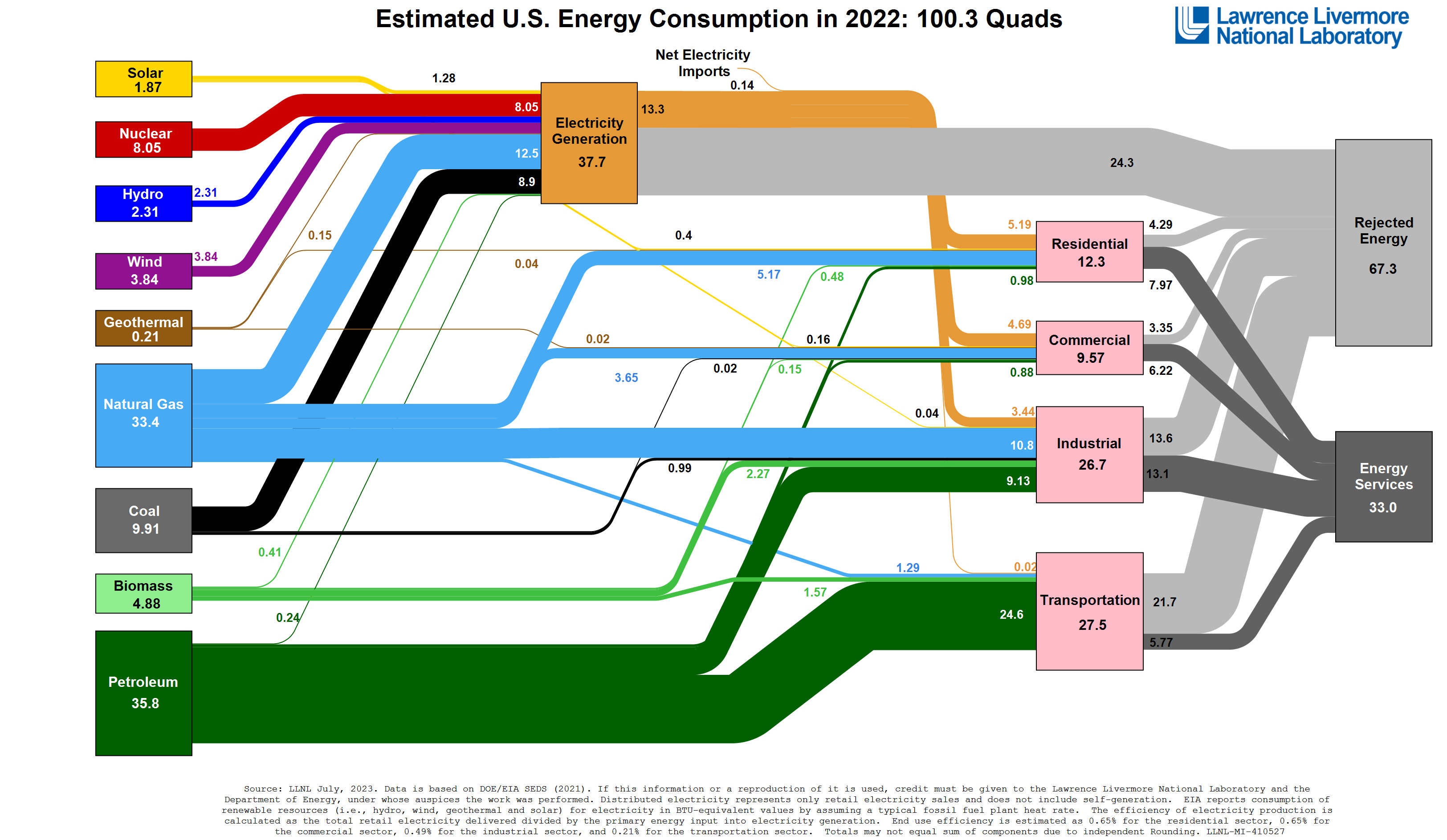
Current global energy production relies heavily on burning fossil fuels. The largest energy sources are oil, coal, and natural gas, all of which are fossil fuels, whereas all non–fossil fuel sources together account for only about 20% of the total. Most oil consumption powers internal combustion engines in cars and trucks, which have a very low efficiency. Only about 25% of all energy input into transportation is used to move vehicles, whereas most of the energy is wasted as heat. Coal is mainly used in power plants to generate electricity, which is also associated with a loss of a little over half. Note that this loss is less than the loss from internal combustion engines, which gives electric cars lower carbon footprints than internal combustion engine cars, even if the electricity is generated from coal. Most natural gas is used to generate electricity and to heat buildings. Hydropower and nuclear power are used exclusively to produce electricity, whereas biomass is used mostly for cooking and heating homes in the developing world. New renewables such as solar and wind supply only a small fraction of all energy.

However, in some countries, renewable energy sources have seen a rapid increase in recent years. Germany, for example, has increased renewables’ contribution to total electricity production from 3% in 1990 to 45% in 2020, while its economy has been one of the strongest in Europe. Denmark plans to move to 100% renewable energy by 2050. In the United States, renewables currently account for 10% of total energy consumption and 15% of electricity production, and it is rapidly increasing. In 2016, for example, the US’s solar power capacity doubled.

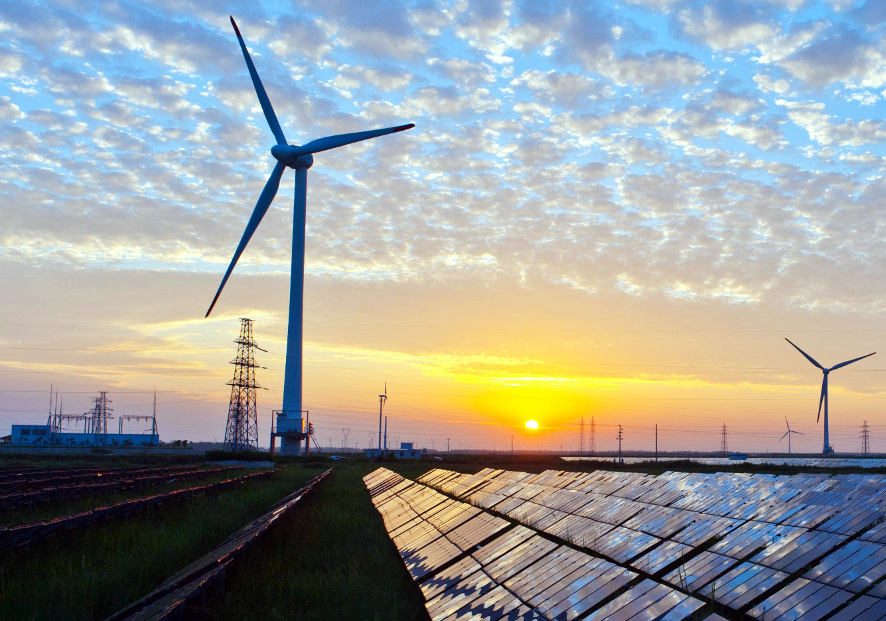
The advantage of renewables is an almost-unlimited potential supply with minimal carbon emissions (some emissions occur during the production and installation of solar panels and wind turbines); in addition, they are not associated with the dangers of nuclear power. Their disadvantage used to be their cost, particularly their high upfront investment cost. Once installed, however, solar panels and wind turbines operate with nearly no maintenance cost since solar energy and wind is free. During the past ten years, the cost for solar panels has decreased by 80%. Thus, if viewed over the lifetime of a system, renewables become competitive with fossil fuels. Other renewable energy sources are geothermal, tide and wave energy, and hydroelectric dams. An issue with renewables is their intermittent energy supply. Solar panels only work during the day, whereas wind turbines only work when the wind blows. However, a recent study showed that 80% of all electricity demand could easily be covered by wind and solar (Shaner et al., 2018).

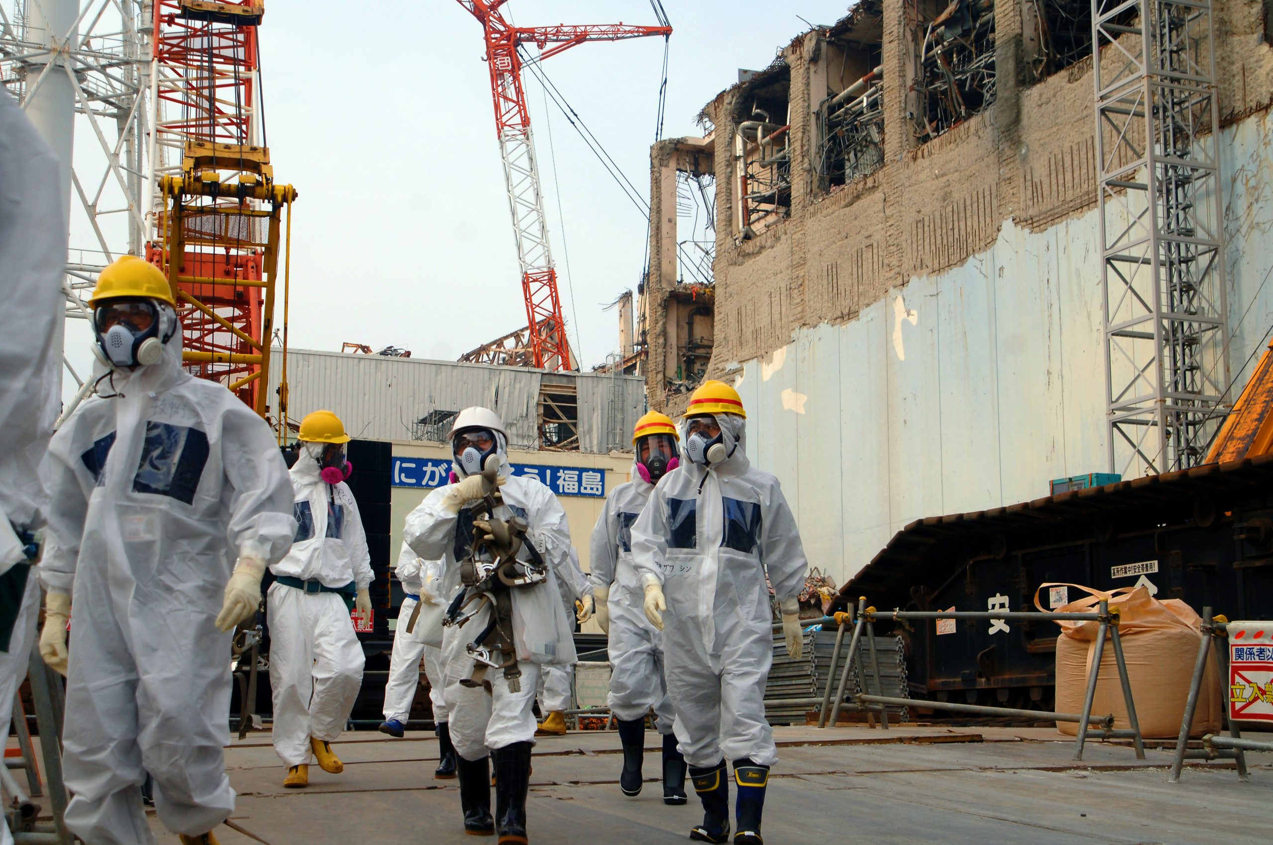
Nuclear plants also provide power that is fossil-free and does not cause carbon emissions (except during construction). For this reason, they are viewed by some as an important future energy source. However, nuclear power has disadvantages too. Not only are their plants expensive to build, they are also dangerous to operate and they produce radioactive waste for which currently no long-term repository exists. Catastrophic accidents—such as the nuclear meltdowns in 2011 at the Japanese Fukushima Daiichi plant and in 1986 at the Chernobyl reactor in what is now northern Ukraine—have shown the dangers associated with nuclear power production. Thus, nuclear power remains a controversial topic.

Currently, many companies are moving toward more electric cars or hybrid vehicles. Due to their much higher efficiencies (80–90%), their energy use is much smaller than for cars with internal combustion engines and their carbon footprint can be close to zero (considering there is some associated with vehicle production) if renewable energy sources are used for the electricity.

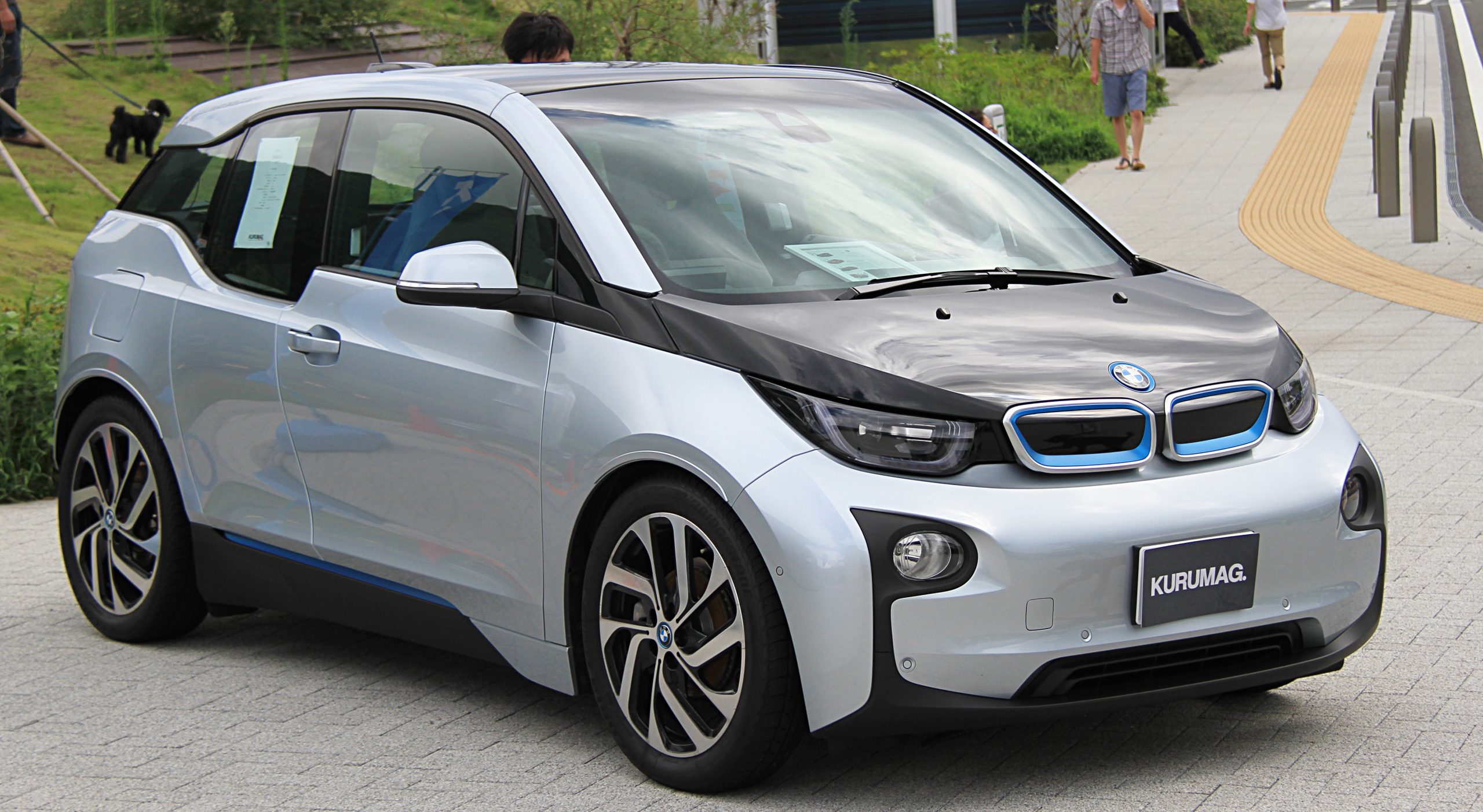
Considering the large amounts of carbon emissions that currently come from the transportation sector and the large losses that occur there, shifting to an electric vehicle fleet could bring a tremendous reduction in future emissions. Even though electric cars are more expensive to purchase, their lifetime costs are lower than gasoline-powered cars. This is because the average cost for equivalent electricity is less than half the cost for a gallon of gas. Electric cars have other advantages too: no oil changes, no pollution, and more torque. Manufacturing electric cars, however, is not without environmental or human impacts, such as from the mining of raw materials used in the production of batteries.

Increasing energy efficiency is another cost-effective way to reduce carbon emissions. Residential and commercial buildings waste about half of their energy. Building insulation not only lowers its carbon emissions but also saves the owner money. Replacing old conventional electrical hot water heaters with inexpensive new heat pump water heaters also reduces electricity use, thereby saving money as well.

15.5.2 International Agreements

In 1992, the United Nations Framework Convention on Climate Change (UNFCCC) was adopted at the Rio Earth Summit. It was ratified by 197 countries (Parties to the Convention). Its Article 2 states:

“The ultimate objective of this Convention and any related legal instruments that the Conference of the Parties may adopt is to achieve, in accordance with the relevant provisions of the Convention, stabilization of greenhouse gas concentrations in the atmosphere at a level that would prevent dangerous anthropogenic interference with the climate system. Such a level should be achieved within a time frame sufficient to allow ecosystems to adapt naturally to climate change, to ensure that food production is not threatened and to enable economic development to proceed in a sustainable manner.”

The UNFCCC recognizes that the developed world is responsible for most historical carbon emissions and thus it should lead the way to reduce its emissions. The annual United Nations Climate Change Conferences, or COPs, are formal gatherings to assess and negotiate climate action, held under the UNFCCC. The Kyoto Protocol, an international agreement linked to the UNFCCC, commits its parties, which are developed countries, to binding carbon emission reduction targets. However, it was not successful in reducing global carbon emissions, presumably at least in part due to the United States never ratifying it, Canada exiting, and Russia not agreeing to emission reductions in its second phase (2013-2020). Under the administration of President George W. Bush, the US argued that it was not fair to reduce US emissions, while China was allowed to increase its emissions, even though per capita emissions in the US were much higher than those in China.

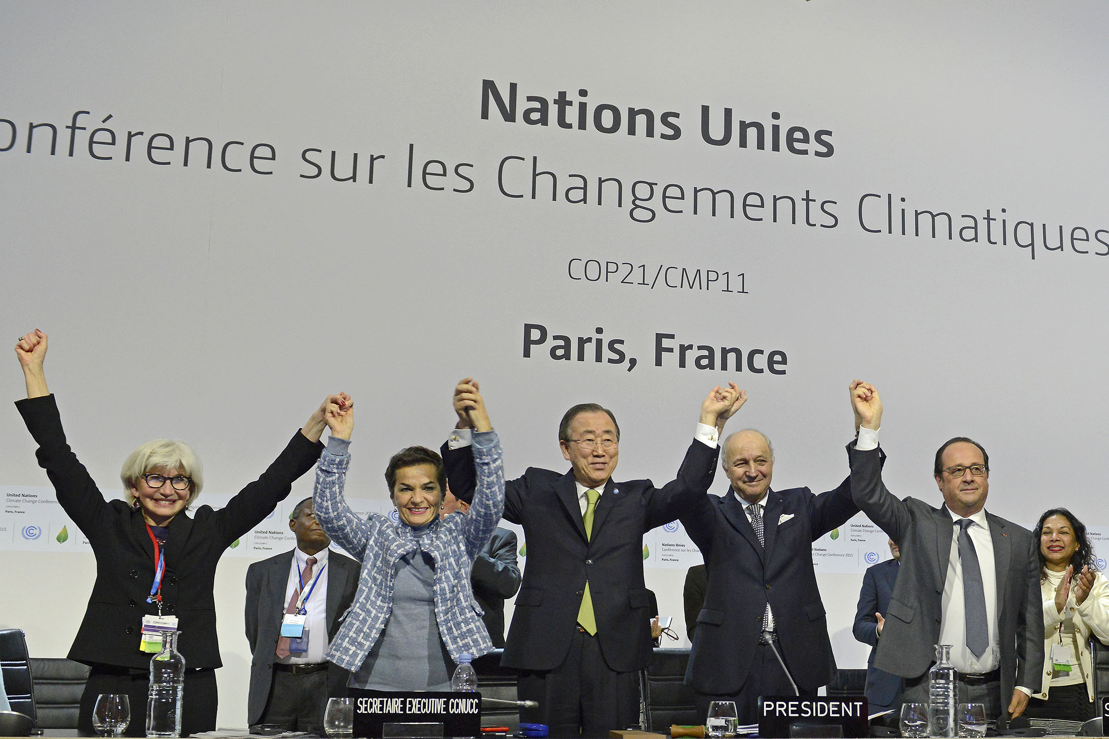
The Paris Agreement has the goal to limit global warming to well below 2°C, and it was ratified by 174 countries. It has made emission reductions essentially voluntary by soliciting pledges from each country and includes developing countries like China. However, resistance against any reduction in carbon emissions was evident when the US administration under President Trump withdrew from the agreement (although the next administration under President Biden re-entered the agreement).

15.5.3 Adaptation and Mitigation

While the situation surrounding global climate change is in serious need of our attention, it is important to realize that many scientists, leaders, and concerned citizens are making solutions to climate change part of their life’s work. The two solutions to the problems caused by climate change are mitigation and adaptation, and we will likely need a combination of both in order to prosper in the future. We know that climate change is already occurring, as we can see and feel the effects of it. For this reason, it is essential to also adapt to our changing environment. This means that we must change our behaviors in response to the changing environment around us.

Adaptation strategies will vary greatly by region, depending on the largest specific impacts in that area. For example, in the city of Delhi, India, a dramatic decrease in rainfall is projected over the next century. This city will likely need to implement policies and practices relating to conservation of water, for example, rainwater harvesting, water re-use, and increased irrigation efficiency. Rain-limited cities near oceans, such as Los Angeles, California, may choose to use desalination to provide drinking water to their citizens. Cities with low elevations near oceans may need to implement adaptation strategies for rising sea levels, from seawalls and levees to relocation of citizens. One adaptation strategy gaining use is the creation or conservation of wetlands, which provide natural protection against storm surges and flooding.

In general, a strategy to mitigate climate change is one that reduces the amount of greenhouse gases in the atmosphere or prevents additional emissions. Mitigation strategies attempt to “fix” the problems caused by climate change. Governmental regulations regarding fuel efficiency of vehicles is one example of an institutionalized mitigation strategy already in place in the United States and in many other countries around the world. Unlike some other countries, there are no carbon taxes or charges on burning fossil fuels in the United States. This is another governmental mitigation strategy that has been shown to be effective in many countries, including India, Japan, France, Costa Rica, Canada, and the United Kingdom.

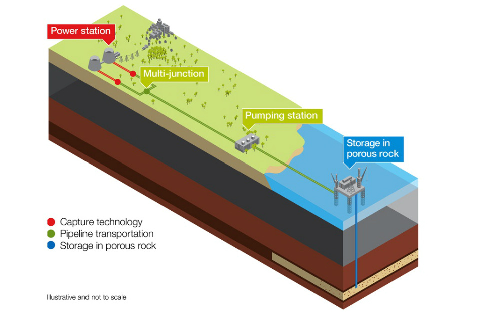
In addition to government measures and incentives, technology can also be harnessed to mitigate climate change. One strategy for this is the use of carbon capture and sequestration (CCS). Through CCS, 80–90% of the CO₂ that would have been emitted to the atmosphere from sources such as a coal-fired power plant is instead captured and then stored deep beneath the Earth’s surface. The CO₂ is often injected and sequestered hundreds of miles underground into porous rock formations sealed below an impermeable layer, where it is stored permanently.

Scientists are also looking into the use of soils and vegetation for carbon storage potential. Proper management of soil and forest ecosystems has been shown to create additional carbon sinks for atmospheric carbon, reducing the overall atmospheric CO₂ burden. Increasing soil carbon further benefits communities by providing better-quality soil for agriculture and cultivation.

Technologies related to alternative energy sources mitigate climate change by providing people with energy not derived from the combustion of fossil fuels. Finally, energy conservation, choosing to walk or bike instead of driving, and disposing of waste properly are simple activities that, when done by large numbers of people, actively mitigate climate change by preventing carbon emissions.

Summary

Included in Earth Science is the study of the system of processes that affect surface environments and atmosphere of the Earth. Recent changes in atmospheric temperature and climate over intervals of decades have been observed. For Earth’s climate to be stable, incoming radiation from the Sun and outgoing radiation from the Sun-warmed Earth must be in balance. Greenhouse gases in the atmosphere absorb the infrared thermal radiation from the Earth’s surface, trapping that heat and warming the atmosphere in a process called the greenhouse effect. Thus, the energy budget is not now in balance and the Earth is warming. Human activity produces many greenhouse gases that have accelerated climate change. CO₂ from fossil fuel burning is one of the major such gases. While the atmosphere is mostly composed of nitrogen and oxygen, the greatest effect on global warming is had by trace components that include greenhouse gases (of which CO₂ and methane are the major examples).

A number of positive feedback mechanisms, processes whose results reinforce the original process, take place in the Earth system. An example of a PFM of great concern is permafrost melting, which causes decay of melting organic material, producing CO₂ and methane (both powerful greenhouse gases) that warm the atmosphere and promote more permafrost melting. Two carbon cycles affect Earth’s atmospheric CO₂ composition, the biologic carbon cycle and the geologic carbon cycle. In the biologic cycle, organisms (mostly plants and also animals that eat them) remove CO₂ from the atmosphere for energy and to build their body tissues and return it to the atmosphere when they die and decay. The biologic cycle is a rapid cycle. In the geologic cycle, some organic matter is preserved in the form of petroleum and coal, while more is dissolved in seawater and captured in carbonate sediments, some of which is subducted into the mantle and returned by volcanic activity. The geologic carbon cycle is slow over geologic time.

Measurements of increasing atmospheric temperature have been made since the nineteenth century, but the upward temperature trend itself increased in the mid-twentieth century, showing the current trend is exponential. Because of the high specific heat of water, the oceans have absorbed most of the added heat. The temporary nature of this storage has been revealed by the record breaking warm years of the recent decade and the increase in intense storms and hurricanes. In 1957, the Mauna Loa CO₂ Observatory was established in Hawai’i, providing constant measurements of atmospheric CO₂ since 1958. The initial value was 315 ppm. The Keeling curve, named for the observatory founder, shows that value has steadily increased exponentially to over 420 ppm now. Compared to proxy data from atmospheric gases trapped in ice cores that show a maximum value for CO₂ of about 300 ppm over the last 800,000 years, the Keeling increase of over 100 ppm in 50 years is dramatic evidence of human-caused CO₂ increase and climate change. As Earth’s temperature rises, glaciers and ice sheets are shrinking, resulting in sea level rise. Atmospheric CO₂ is also absorbed in seawater, producing increased concentrations of carbonic acid, which is raising the pH of the oceans, making it harder for marine life to extract carbonate for their skeletal materials.

Earth’s climate has changed over geologic time with periods of major glaciations. There was a high temperature period in the Mesozoic shown by fossils in high latitudes and the Western Interior Seaway covering what is now the Midwest. However, climate has been cooling during the Cenozoic culminating in the most recent ice age. Since the ice age, several proxy indicators of ancient climate show that the rate and amount of current climate change is unique in geologic history and can only be attributed to human activity.

Addressing climate change is a challenging task, largely because our industrialized society has relied heavily on fossil fuels for energy and this dependency continues today. To stabilize the climate, we must aim for near-zero carbon emissions in the long term. Given the global nature of the problem, international cooperation is essential. Additionally, since some degree of climate change is inevitable, we must also prepare to adapt to its impacts.